Linear Modeling Assignment: Data Analysis and Model Building

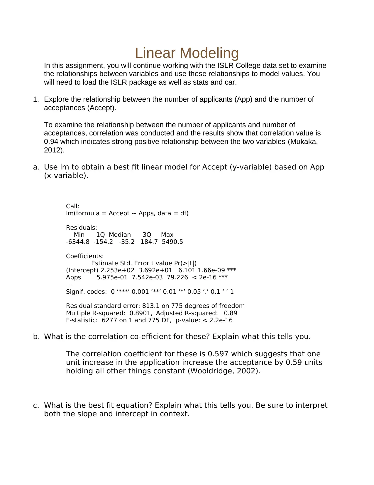
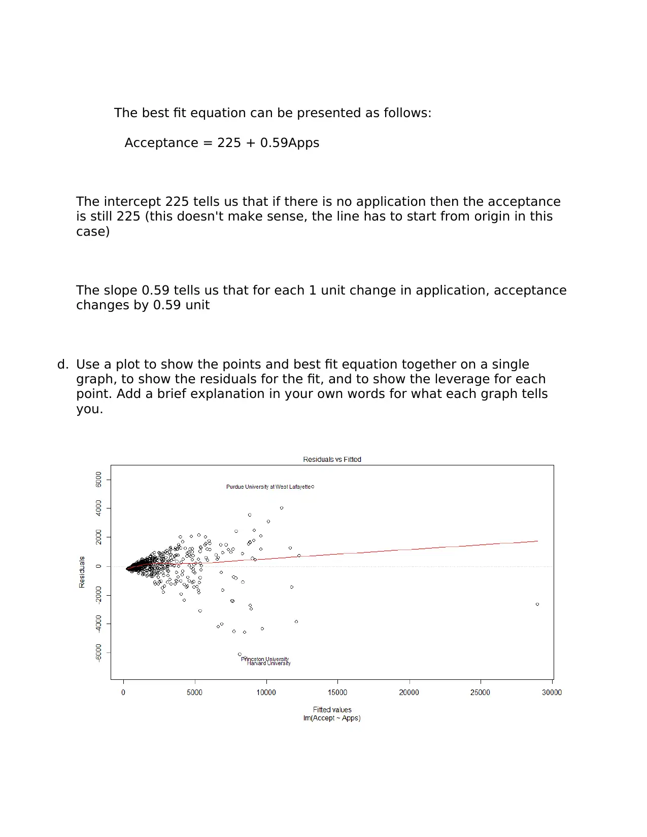
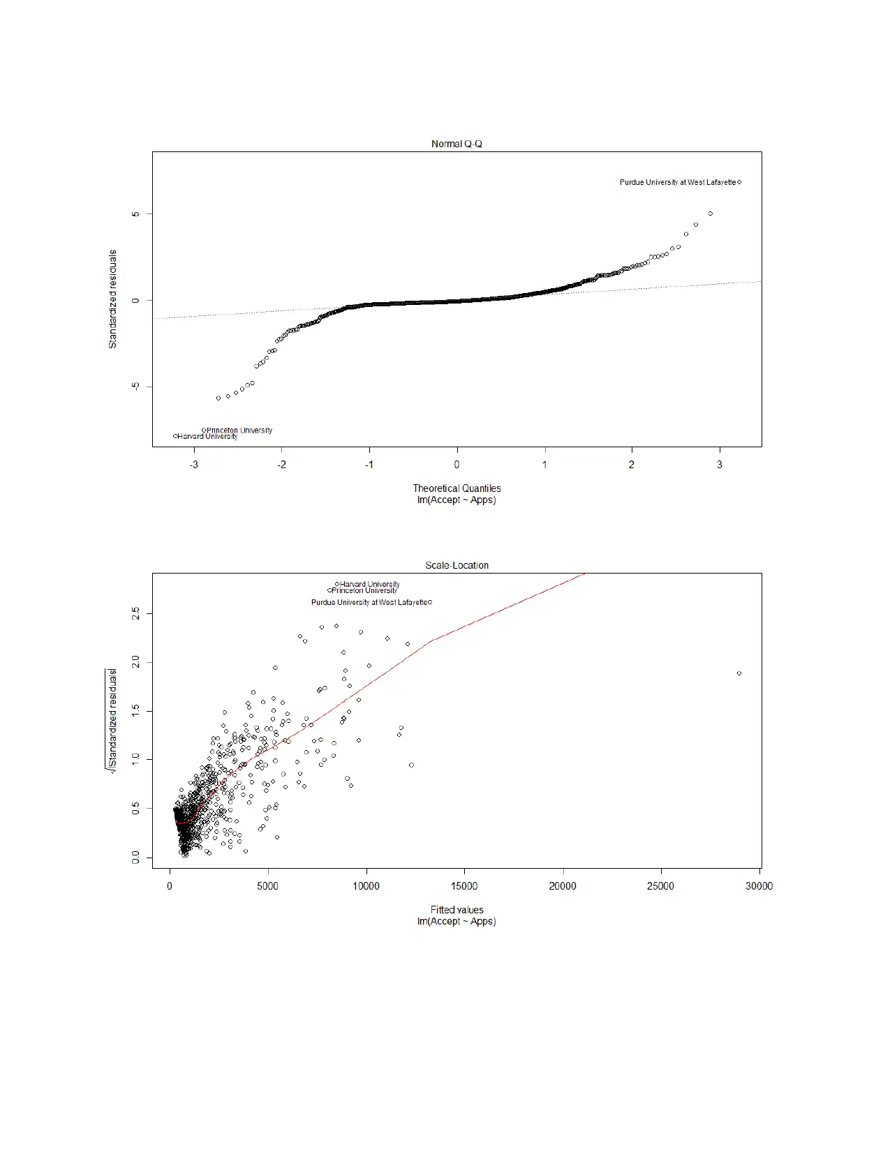
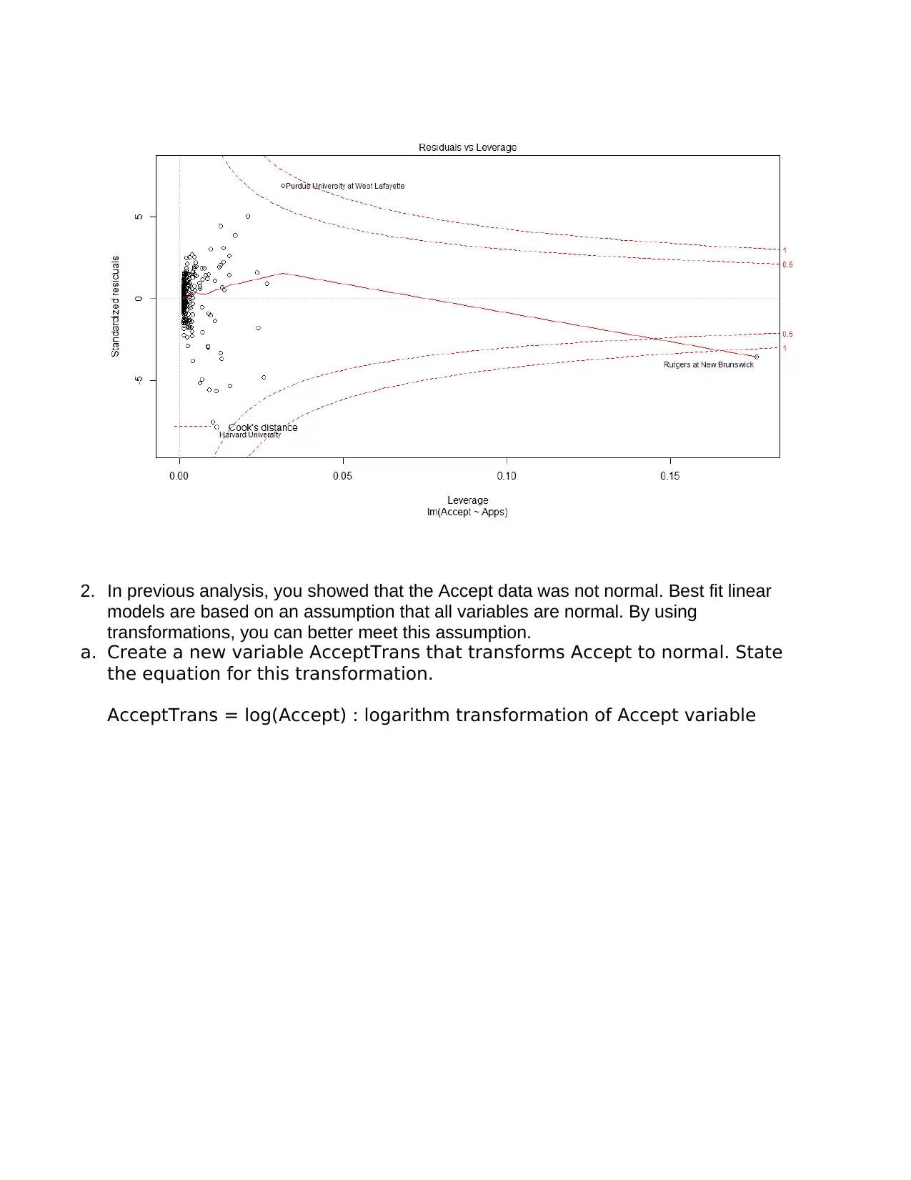
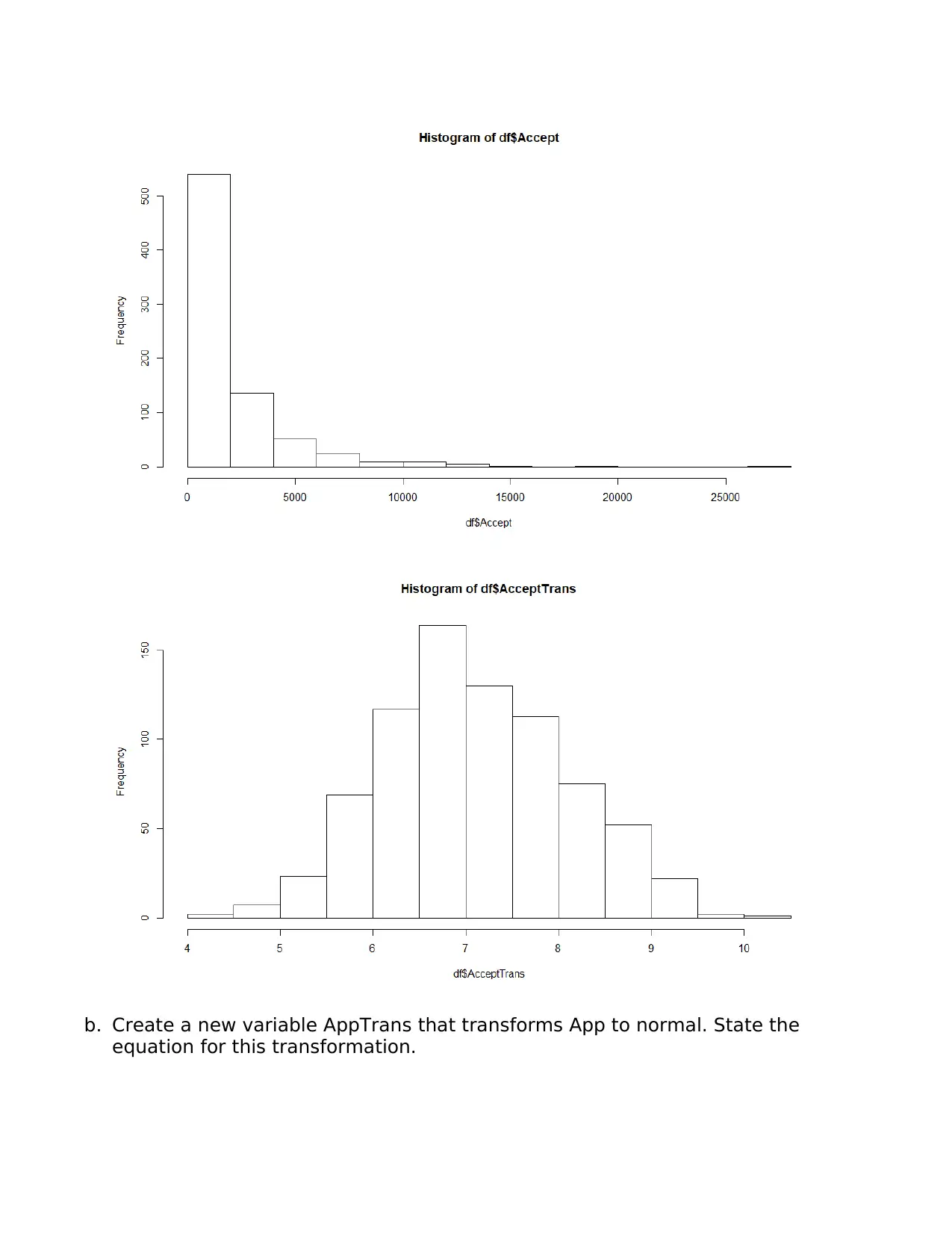
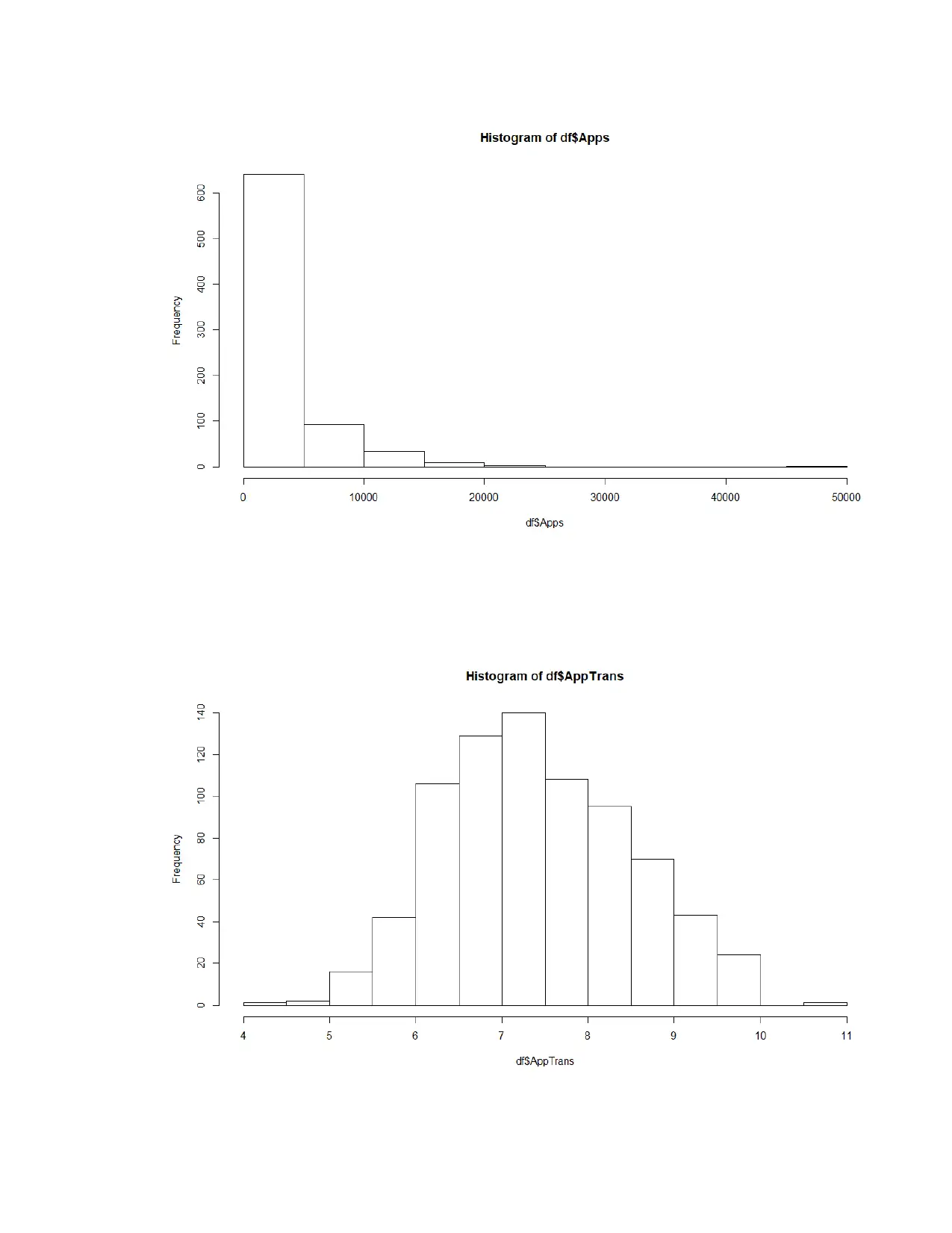
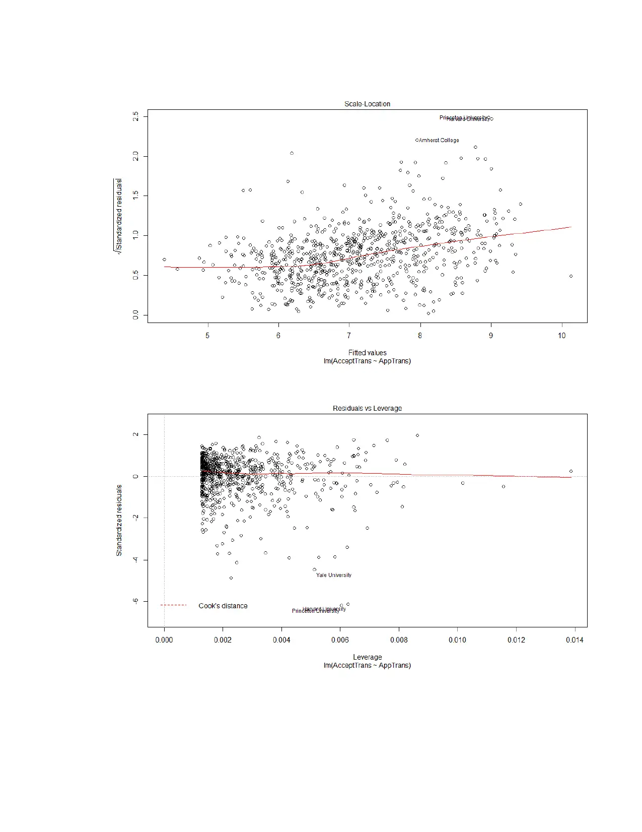
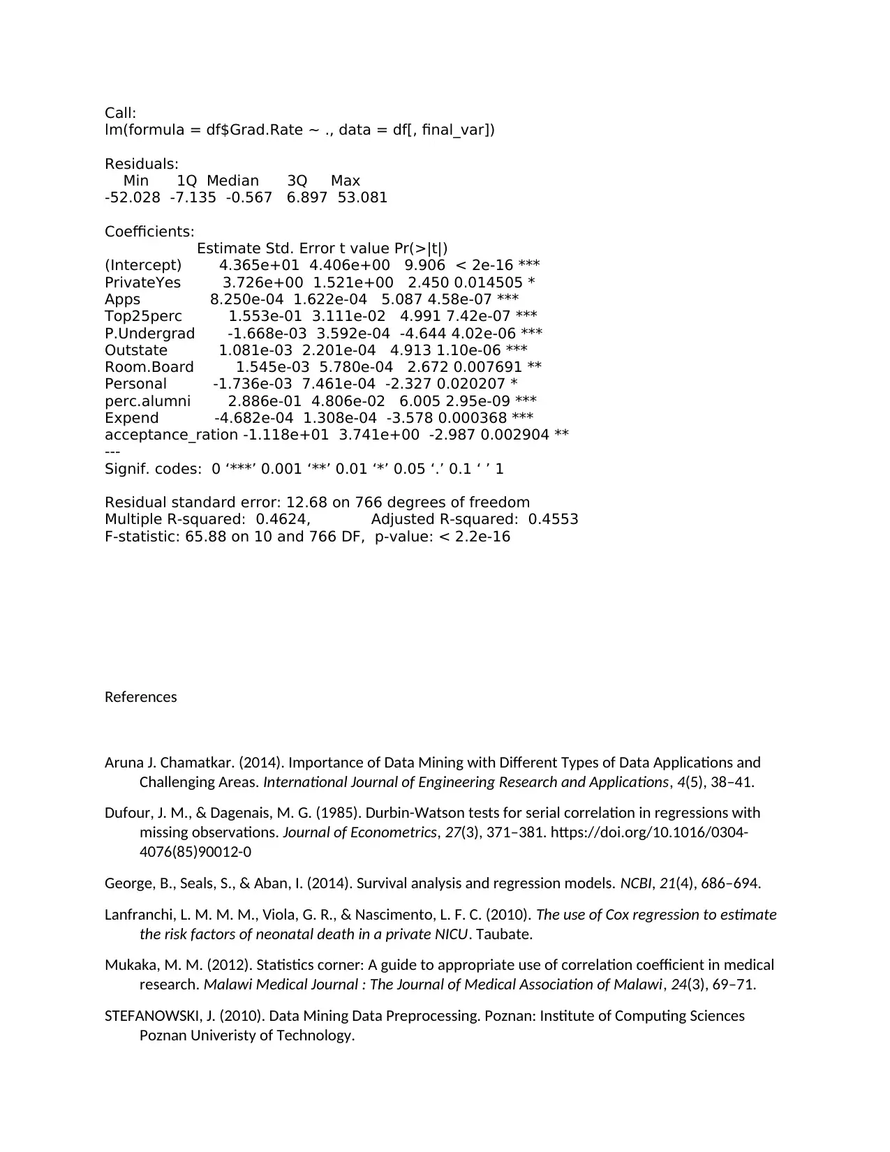
This assignment delves into linear modeling using the ISLR College dataset. It begins by examining the relationship between the number of applicants and acceptances, calculating the correlation coefficient, and constructing a best-fit linear model. The assignment explores the interpretation of the model's equation, including the intercept and slope. It then addresses the non-normality of the data by applying transformations to both the acceptance and application variables to meet the assumptions of linear regression. The analysis includes a second linear model using the transformed variables, alongside an analysis of the assumptions of linear regression. Finally, the assignment concludes with the creation of a model to predict the graduation rate based on various college-related variables, emphasizing the process of model building, variable selection, and the evaluation of the final model's fit. The student utilizes R programming language and statistical concepts throughout the assignment.

Linear Modeling
In this assignment, you will continue working with the ISLR College data set to examine
the relationships between variables and use these relationships to model values. You
will need to load the ISLR package as well as stats and car.
1. Explore the relationship between the number of applicants (App) and the number of
acceptances (Accept).
To examine the relationship between the number of applicants and number of
acceptances, correlation was conducted and the results show that correlation value is
0.94 which indicates strong positive relationship between the two variables (Mukaka,
2012).
a. Use lm to obtain a best fit linear model for Accept (y-variable) based on App
(x-variable).
Call:
lm(formula = Accept ~ Apps, data = df)
Residuals:
Min 1Q Median 3Q Max
-6344.8 -154.2 -35.2 184.7 5490.5
Coefficients:
Estimate Std. Error t value Pr(>|t|)
(Intercept) 2.253e+02 3.692e+01 6.101 1.66e-09 ***
Apps 5.975e-01 7.542e-03 79.226 < 2e-16 ***
---
Signif. codes: 0 ‘***’ 0.001 ‘**’ 0.01 ‘*’ 0.05 ‘.’ 0.1 ‘ ’ 1
Residual standard error: 813.1 on 775 degrees of freedom
Multiple R-squared: 0.8901, Adjusted R-squared: 0.89
F-statistic: 6277 on 1 and 775 DF, p-value: < 2.2e-16
b. What is the correlation co-efficient for these? Explain what this tells you.
The correlation coefficient for these is 0.597 which suggests that one
unit increase in the application increase the acceptance by 0.59 units
holding all other things constant (Wooldridge, 2002).
c. What is the best fit equation? Explain what this tells you. Be sure to interpret
both the slope and intercept in context.

The best fit equation can be presented as follows:
Acceptance = 225 + 0.59Apps
The intercept 225 tells us that if there is no application then the acceptance
is still 225 (this doesn't make sense, the line has to start from origin in this
case)
The slope 0.59 tells us that for each 1 unit change in application, acceptance
changes by 0.59 unit
d. Use a plot to show the points and best fit equation together on a single
graph, to show the residuals for the fit, and to show the leverage for each
point. Add a brief explanation in your own words for what each graph tells
you.

2. In previous analysis, you showed that the Accept data was not normal. Best fit linear
models are based on an assumption that all variables are normal. By using
transformations, you can better meet this assumption.
a. Create a new variable AcceptTrans that transforms Accept to normal. State
the equation for this transformation.
AcceptTrans = log(Accept) : logarithm transformation of Accept variable

b. Create a new variable AppTrans that transforms App to normal. State the
equation for this transformation.

c. Use lm to obtain a best fit linear model for AcceptTrans (y-variable) based on
AppTrans (x-variable).
Call:
lm(formula = AcceptTrans ~ AppTrans, data = df)
Residuals:
Min 1Q Median 3Q Max
-1.34359 -0.08541 0.04058 0.13561 0.42310
Coefficients:
Estimate Std. Error t value Pr(>|t|)
(Intercept) 0.428867 0.054618 7.852 1.36e-14 ***
AppTrans 0.899579 0.007279 123.590 < 2e-16 ***
---
d. What is the correlation co-efficient for these? Explain what this tells you.
The correlation coefficient: 0.89, This means when application increases by
1%, acceptance increases by 0.89%
e. What is the best fit equation? Explain what this tells you. Be sure to interpret
both the slope and intercept in context.
Best fit: AcceptTrans = 0.42 + 0.899AppTrans
The intercept 0.42 tells us that if there is no application then the
acceptance is still 0.42 (this doesn't make sense, the line has to start
from origin in this case) (George, Seals, & Aban, 2014; Lanfranchi,
Viola, & Nascimento, 2010)
The slope 0.89 tells us that , for each 1% change in application,
acceptance changes by 0.89%
f. Use a plot to show the points and best fit equation together on a single
graph, to show the residuals for the fit, and to show the leverage for each
point. Add a brief explanation in your own words for what each graph tells
you.

3. Describe each of the assumptions for linear regression. Are each of these met in your
first model? Are each of these met in your second model?
Assumptions:
i. The target variable has to be normally distributed. Independent variable is not
necessarily needs to be normally distributed but it gives best results when it is
The first model doesn’t satisfy the above assumptions while the second model satisfy
the above assumption.
ii. Multicollinearity
Since it is only a single independent variable, there will not be a problem of
multicollinearity (Dufour & Dagenais, 1985) (Aruna J. Chamatkar, 2014;
STEFANOWSKI, 2010)
iii. Heteroscedasticity
4. You want a model to predict graduation rate (Grad.Rate) based on one or more of the
other variables in the College data set. Create and characterize a model for Grad.Rate.
You may consider single variable or multi-variate models. You may incorporate normal
transformations if desired. You may use cross terms if desired. You may consider
polynomial, exponential, or other terms if desired. The goal is to explore modeling
capabilities in R and describe your understanding of modeling procedures and
techniques. Include in your submission a description of your modeling processes, the
equation for the final model you created, and a characterization of the fit of that model.
Ans:
i. Step 1: Include all variables in the model
ii. Step 2: Check the significance of the variable, drop if it is insignificant
iii. Step 2: Check vif & remove the variable with high vif
iv. Step 3: Iterate the process until all the variables are significant & the vif is in control
(<10)
Final model:

Call:
lm(formula = df$Grad.Rate ~ ., data = df[, final_var])
Residuals:
Min 1Q Median 3Q Max
-52.028 -7.135 -0.567 6.897 53.081
Coefficients:
Estimate Std. Error t value Pr(>|t|)
(Intercept) 4.365e+01 4.406e+00 9.906 < 2e-16 ***
PrivateYes 3.726e+00 1.521e+00 2.450 0.014505 *
Apps 8.250e-04 1.622e-04 5.087 4.58e-07 ***
Top25perc 1.553e-01 3.111e-02 4.991 7.42e-07 ***
P.Undergrad -1.668e-03 3.592e-04 -4.644 4.02e-06 ***
Outstate 1.081e-03 2.201e-04 4.913 1.10e-06 ***
Room.Board 1.545e-03 5.780e-04 2.672 0.007691 **
Personal -1.736e-03 7.461e-04 -2.327 0.020207 *
perc.alumni 2.886e-01 4.806e-02 6.005 2.95e-09 ***
Expend -4.682e-04 1.308e-04 -3.578 0.000368 ***
acceptance_ration -1.118e+01 3.741e+00 -2.987 0.002904 **
---
Signif. codes: 0 ‘***’ 0.001 ‘**’ 0.01 ‘*’ 0.05 ‘.’ 0.1 ‘ ’ 1
Residual standard error: 12.68 on 766 degrees of freedom
Multiple R-squared: 0.4624, Adjusted R-squared: 0.4553
F-statistic: 65.88 on 10 and 766 DF, p-value: < 2.2e-16
References
Aruna J. Chamatkar. (2014). Importance of Data Mining with Different Types of Data Applications and
Challenging Areas. International Journal of Engineering Research and Applications, 4(5), 38–41.
Dufour, J. M., & Dagenais, M. G. (1985). Durbin-Watson tests for serial correlation in regressions with
missing observations. Journal of Econometrics, 27(3), 371–381. https://doi.org/10.1016/0304-
4076(85)90012-0
George, B., Seals, S., & Aban, I. (2014). Survival analysis and regression models. NCBI, 21(4), 686–694.
Lanfranchi, L. M. M. M., Viola, G. R., & Nascimento, L. F. C. (2010). The use of Cox regression to estimate
the risk factors of neonatal death in a private NICU. Taubate.
Mukaka, M. M. (2012). Statistics corner: A guide to appropriate use of correlation coefficient in medical
research. Malawi Medical Journal : The Journal of Medical Association of Malawi, 24(3), 69–71.
STEFANOWSKI, J. (2010). Data Mining Data Preprocessing. Poznan: Institute of Computing Sciences
Poznan Univeristy of Technology.

Wooldridge, J. M. (2002). Econometric Analysis of Cross Section and Panel Data. booksgooglecom (Vol.
58). MIT Press. https://doi.org/10.1515/humr.2003.021