Solution to Linear Optimization and Decision Making Problems
VerifiedAdded on 2023/04/22
|12
|2309
|453
Homework Assignment
AI Summary
This assignment provides solutions to linear optimization and decision-making problems. It includes a linear optimization model for maximizing profit in a desk production scenario, analyzing constraints, shadow prices, and optimal production quantities. The solution also addresses an unbounded feasible region problem, determining corner points and minimized cost. Furthermore, it examines deceleration versus distance, verifying the Central Limit Theorem for sample means, and calculating Expected Monetary Values (EMV) for different decision strategies, including the Expected Value of Perfect Information (EVPI). The analysis incorporates relevant references and detailed calculations to support the findings.

1
Linear Optimization and Decision Making Problems
Linear Optimization and Decision Making Problems
Paraphrase This Document
Need a fresh take? Get an instant paraphrase of this document with our AI Paraphraser

2
Answer 1 Part a
Let X units of standard desks and Y unit of deluxe desks will be produced in next week.
Then the objective is to maximize the profit which will be yield by selling these desks in next
week (Vanderbei, 2014).
Hence, the objective function is Max Z= 150 * X+ 320 *Y
The constraints are of less than equal to type. There will be three constraints, one for labour
hours, then for pine requirement and finally for oak requirement.
The three constraints are,
LABOUR (Hours) 10*X+16*Y ≤ 400
PINE (Square feet) 80*X+60*Y ≤ 5000
OAK (Square feet) 18*Y ≤ 750
The non-negative constraints are X ≥ 0 and Y ≥ 0.
Answer 1 Part b
1. The shadow price for labour hours is non zero. Therefore labour hour constraint is the
only Binding constraint (Munier, Hontoria, & Jiménez-Sáez, 2019).
2. Maximize profit will be Max Z= 150 * X (=0) + 320 *Y (= 25) = $ 8000
3. Slack values for
Pine = 5000- 1500 = 3500,
Oak = 750 -450 = 300, and
Labor = 400 – 400 = 0 (Binding constraint).
3
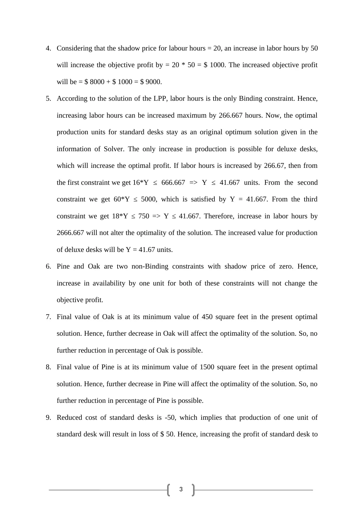
4. Considering that the shadow price for labour hours = 20, an increase in labor hours by 50
will increase the objective profit by = 20 * 50 = $ 1000. The increased objective profit
will be = $ 8000 + $ 1000 = $ 9000.
5. According to the solution of the LPP, labor hours is the only Binding constraint. Hence,
increasing labor hours can be increased maximum by 266.667 hours. Now, the optimal
production units for standard desks stay as an original optimum solution given in the
information of Solver. The only increase in production is possible for deluxe desks,
which will increase the optimal profit. If labor hours is increased by 266.67, then from
the first constraint we get 16*Y ≤ 666.667 => Y ≤ 41.667 units. From the second
constraint we get 60*Y ≤ 5000, which is satisfied by Y = 41.667. From the third
constraint we get 18*Y ≤ 750 => Y ≤ 41.667. Therefore, increase in labor hours by
2666.667 will not alter the optimality of the solution. The increased value for production
of deluxe desks will be Y = 41.67 units.
6. Pine and Oak are two non-Binding constraints with shadow price of zero. Hence,
increase in availability by one unit for both of these constraints will not change the
objective profit.
7. Final value of Oak is at its minimum value of 450 square feet in the present optimal
solution. Hence, further decrease in Oak will affect the optimality of the solution. So, no
further reduction in percentage of Oak is possible.
8. Final value of Pine is at its minimum value of 1500 square feet in the present optimal
solution. Hence, further decrease in Pine will affect the optimality of the solution. So, no
further reduction in percentage of Pine is possible.
9. Reduced cost of standard desks is -50, which implies that production of one unit of
standard desk will result in loss of $ 50. Hence, increasing the profit of standard desk to
⊘ This is a preview!⊘
Do you want full access?
Subscribe today to unlock all pages.
Trusted by 1+ million students worldwide
4
at least $ 200 is possible without changing the optimal solution. But, to produce positive
units of standard desks, the profit for one standard desk should be greater than $ 200.
Answer 2
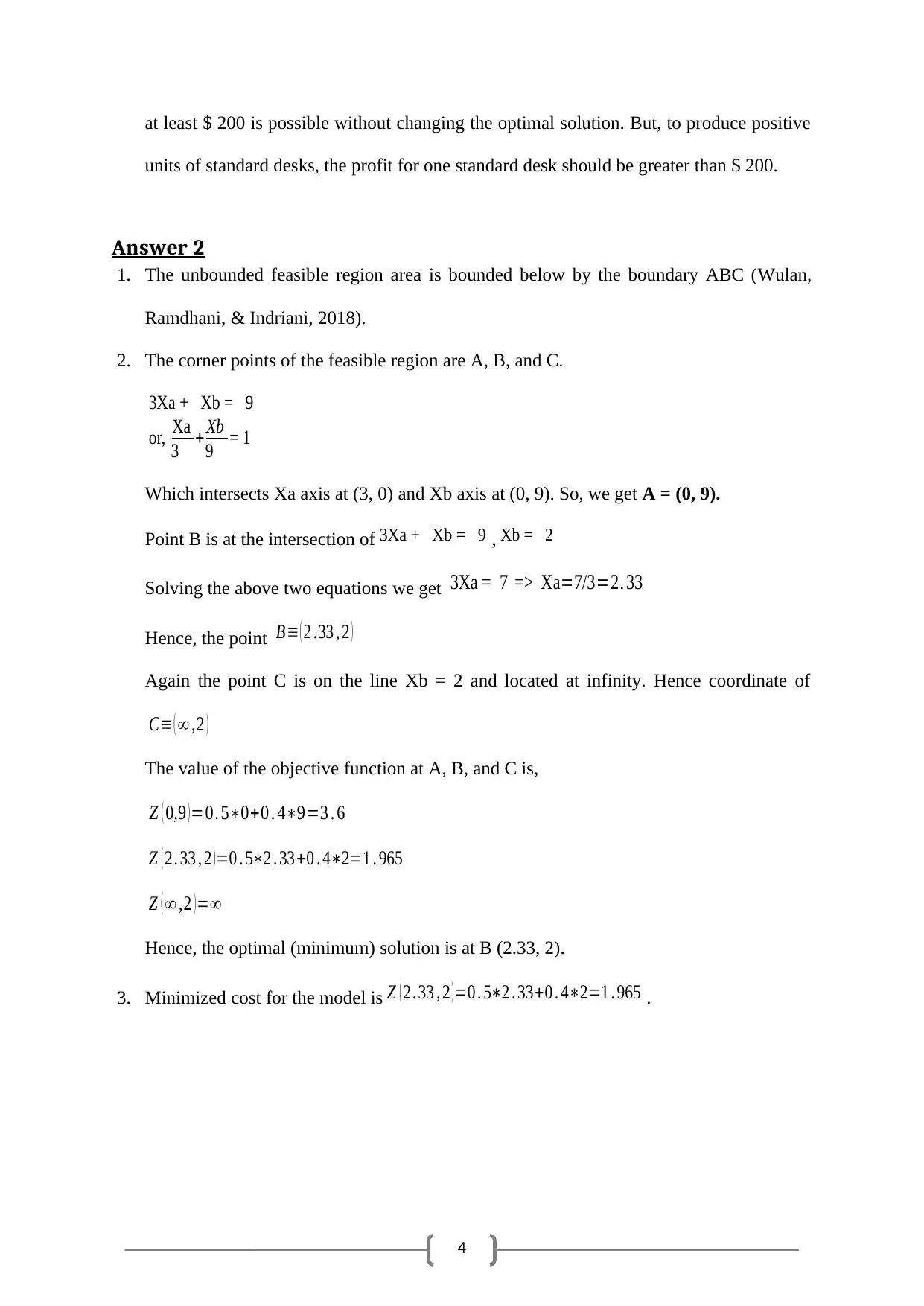
1. The unbounded feasible region area is bounded below by the boundary ABC (Wulan,
Ramdhani, & Indriani, 2018).
2. The corner points of the feasible region are A, B, and C.
3Xa + Xb = 9
or, Xa
3 + Xb
9 = 1
Which intersects Xa axis at (3, 0) and Xb axis at (0, 9). So, we get A = (0, 9).
Point B is at the intersection of 3Xa + Xb = 9 , Xb = 2
Solving the above two equations we get 3Xa = 7 => Xa=7/3=2. 33
Hence, the point B≡ ( 2 .33 , 2 )
Again the point C is on the line Xb = 2 and located at infinity. Hence coordinate of
C≡ ( ∞ ,2 )
The value of the objective function at A, B, and C is,
Z ( 0,9 ) =0. 5∗0+0 . 4∗9=3 . 6
Z ( 2. 33 , 2 ) =0 . 5∗2 . 33+0 . 4∗2=1 . 965
Z ( ∞ ,2 ) =∞
Hence, the optimal (minimum) solution is at B (2.33, 2).
3. Minimized cost for the model is Z ( 2. 33 , 2 ) =0 . 5∗2 . 33+0 . 4∗2=1 . 965 .
at least $ 200 is possible without changing the optimal solution. But, to produce positive
units of standard desks, the profit for one standard desk should be greater than $ 200.
Answer 2
1. The unbounded feasible region area is bounded below by the boundary ABC (Wulan,
Ramdhani, & Indriani, 2018).
2. The corner points of the feasible region are A, B, and C.
3Xa + Xb = 9
or, Xa
3 + Xb
9 = 1
Which intersects Xa axis at (3, 0) and Xb axis at (0, 9). So, we get A = (0, 9).
Point B is at the intersection of 3Xa + Xb = 9 , Xb = 2
Solving the above two equations we get 3Xa = 7 => Xa=7/3=2. 33
Hence, the point B≡ ( 2 .33 , 2 )
Again the point C is on the line Xb = 2 and located at infinity. Hence coordinate of
C≡ ( ∞ ,2 )
The value of the objective function at A, B, and C is,
Z ( 0,9 ) =0. 5∗0+0 . 4∗9=3 . 6
Z ( 2. 33 , 2 ) =0 . 5∗2 . 33+0 . 4∗2=1 . 965
Z ( ∞ ,2 ) =∞
Hence, the optimal (minimum) solution is at B (2.33, 2).
3. Minimized cost for the model is Z ( 2. 33 , 2 ) =0 . 5∗2 . 33+0 . 4∗2=1 . 965 .
Paraphrase This Document
Need a fresh take? Get an instant paraphrase of this document with our AI Paraphraser
5
Answer 3
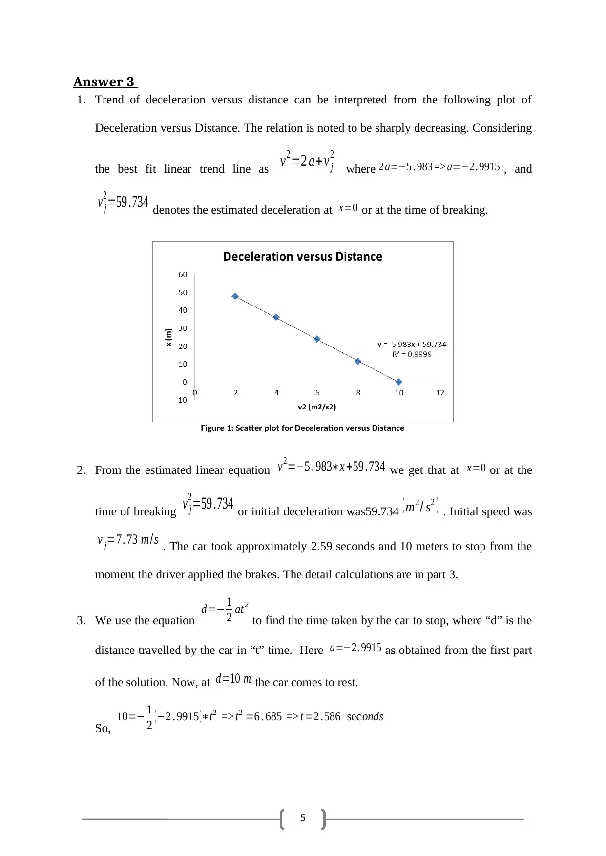
1. Trend of deceleration versus distance can be interpreted from the following plot of
Deceleration versus Distance. The relation is noted to be sharply decreasing. Considering
the best fit linear trend line as v2=2 a+ v j
2
where 2 a=−5 . 983 => a=−2. 9915 , and
v j
2=59 .734 denotes the estimated deceleration at x=0 or at the time of breaking.
Figure 1: Scatter plot for Deceleration versus Distance
2. From the estimated linear equation v2=−5 . 983∗x +59 .734 we get that at x=0 or at the
time of breaking v j
2=59 .734 or initial deceleration was59.734 ( m2/ s2 ) . Initial speed was
v j=7. 73 m/ s . The car took approximately 2.59 seconds and 10 meters to stop from the
moment the driver applied the brakes. The detail calculations are in part 3.
3. We use the equation d=− 1
2 at2
to find the time taken by the car to stop, where “d” is the
distance travelled by the car in “t” time. Here a=−2. 9915 as obtained from the first part
of the solution. Now, at d=10 m the car comes to rest.
So, 10=− 1
2 ( −2 . 9915 )∗t2 => t2 =6 . 685 => t=2 .586 sec onds
Answer 3
1. Trend of deceleration versus distance can be interpreted from the following plot of
Deceleration versus Distance. The relation is noted to be sharply decreasing. Considering
the best fit linear trend line as v2=2 a+ v j
2
where 2 a=−5 . 983 => a=−2. 9915 , and
v j
2=59 .734 denotes the estimated deceleration at x=0 or at the time of breaking.
Figure 1: Scatter plot for Deceleration versus Distance
2. From the estimated linear equation v2=−5 . 983∗x +59 .734 we get that at x=0 or at the
time of breaking v j
2=59 .734 or initial deceleration was59.734 ( m2/ s2 ) . Initial speed was
v j=7. 73 m/ s . The car took approximately 2.59 seconds and 10 meters to stop from the
moment the driver applied the brakes. The detail calculations are in part 3.
3. We use the equation d=− 1
2 at2
to find the time taken by the car to stop, where “d” is the
distance travelled by the car in “t” time. Here a=−2. 9915 as obtained from the first part
of the solution. Now, at d=10 m the car comes to rest.
So, 10=− 1
2 ( −2 . 9915 )∗t2 => t2 =6 . 685 => t=2 .586 sec onds
6
Hence, the car comes to rest in approximately 2.59 seconds from position of applying the
brakes.
Answer 4
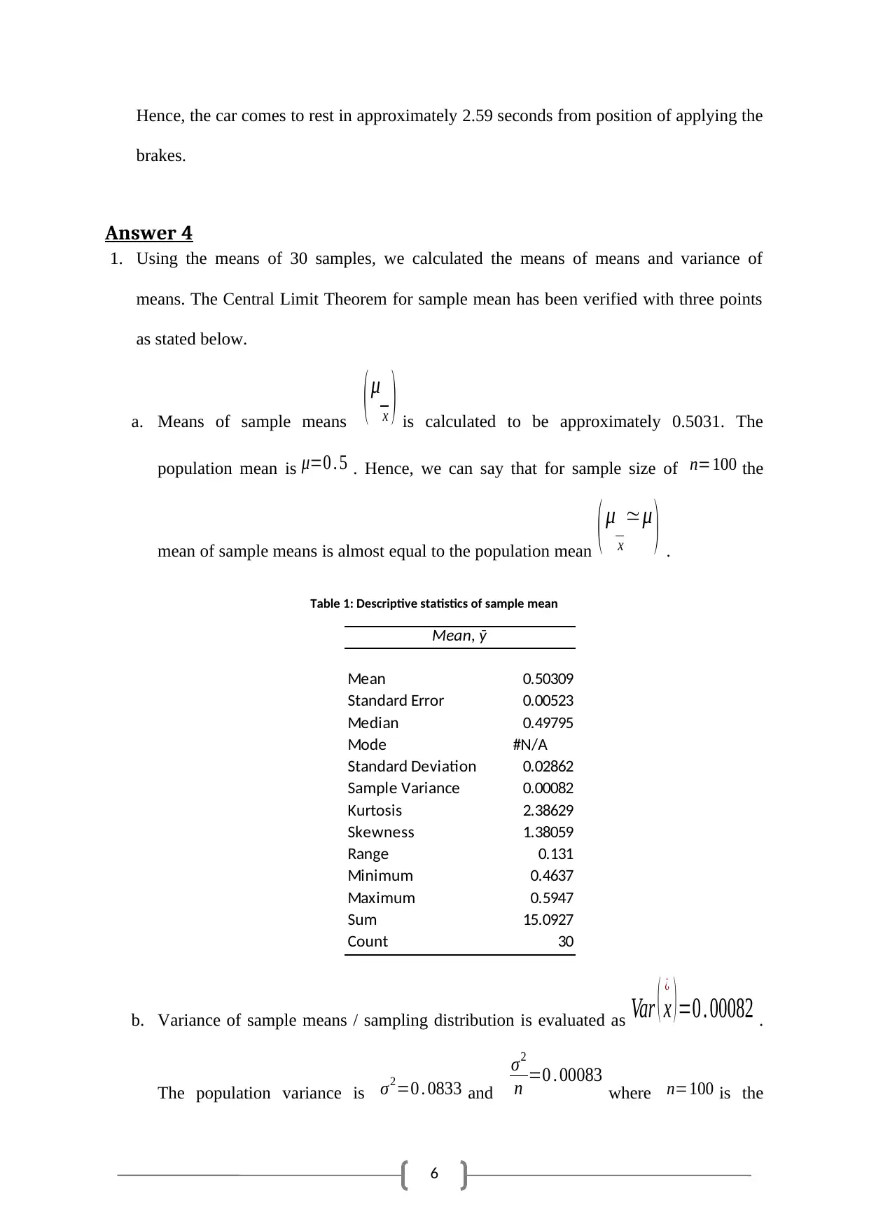
1. Using the means of 30 samples, we calculated the means of means and variance of
means. The Central Limit Theorem for sample mean has been verified with three points
as stated below.
a. Means of sample means ( μ
x ) is calculated to be approximately 0.5031. The
population mean is μ=0 . 5 . Hence, we can say that for sample size of n=100 the
mean of sample means is almost equal to the population mean ( μ
x
≃μ ) .
Table 1: Descriptive statistics of sample mean
Mean, ȳ
Mean 0.50309
Standard Error 0.00523
Median 0.49795
Mode #N/A
Standard Deviation 0.02862
Sample Variance 0.00082
Kurtosis 2.38629
Skewness 1.38059
Range 0.131
Minimum 0.4637
Maximum 0.5947
Sum 15.0927
Count 30
b. Variance of sample means / sampling distribution is evaluated as Var ( x
¿
) =0 . 00082 .
The population variance is σ2=0 . 0833 and
σ2
n =0 . 00083 where n=100 is the
Hence, the car comes to rest in approximately 2.59 seconds from position of applying the
brakes.
Answer 4
1. Using the means of 30 samples, we calculated the means of means and variance of
means. The Central Limit Theorem for sample mean has been verified with three points
as stated below.
a. Means of sample means ( μ
x ) is calculated to be approximately 0.5031. The
population mean is μ=0 . 5 . Hence, we can say that for sample size of n=100 the
mean of sample means is almost equal to the population mean ( μ
x
≃μ ) .
Table 1: Descriptive statistics of sample mean
Mean, ȳ
Mean 0.50309
Standard Error 0.00523
Median 0.49795
Mode #N/A
Standard Deviation 0.02862
Sample Variance 0.00082
Kurtosis 2.38629
Skewness 1.38059
Range 0.131
Minimum 0.4637
Maximum 0.5947
Sum 15.0927
Count 30
b. Variance of sample means / sampling distribution is evaluated as Var ( x
¿
) =0 . 00082 .
The population variance is σ2=0 . 0833 and
σ2
n =0 . 00083 where n=100 is the
⊘ This is a preview!⊘
Do you want full access?
Subscribe today to unlock all pages.
Trusted by 1+ million students worldwide
7
sample size of each of the 30 samples. Therefore,
Var ( x
¿
) =0 . 00082≃ σ2
n proves that
variance of the sampling distribution is consistent to
σ2
n for considerably large sample
size.
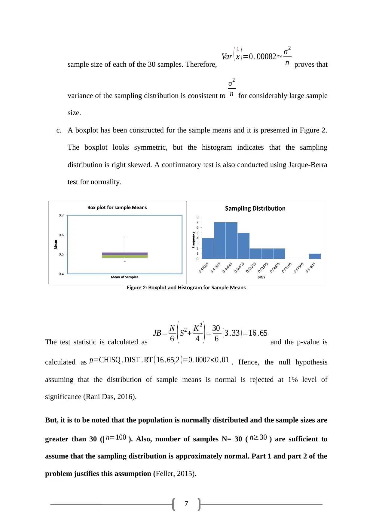
c. A boxplot has been constructed for the sample means and it is presented in Figure 2.
The boxplot looks symmetric, but the histogram indicates that the sampling
distribution is right skewed. A confirmatory test is also conducted using Jarque-Berra
test for normality.
Figure 2: Boxplot and Histogram for Sample Means
The test statistic is calculated as
JB= N
6 ( S2+ K2
4 ) =30
6 ( 3 .33 ) =16 .65
and the p-value is
calculated as p=CHISQ . DIST . RT(16 .65,2 )=0 . 0002<0 .01 . Hence, the null hypothesis
assuming that the distribution of sample means is normal is rejected at 1% level of
significance (Rani Das, 2016).
But, it is to be noted that the population is normally distributed and the sample sizes are
greater than 30 (| n=100 ). Also, number of samples N= 30 ( n≥30 ) are sufficient to
assume that the sampling distribution is approximately normal. Part 1 and part 2 of the
problem justifies this assumption (Feller, 2015).
sample size of each of the 30 samples. Therefore,
Var ( x
¿
) =0 . 00082≃ σ2
n proves that
variance of the sampling distribution is consistent to
σ2
n for considerably large sample
size.
c. A boxplot has been constructed for the sample means and it is presented in Figure 2.
The boxplot looks symmetric, but the histogram indicates that the sampling
distribution is right skewed. A confirmatory test is also conducted using Jarque-Berra
test for normality.
Figure 2: Boxplot and Histogram for Sample Means
The test statistic is calculated as
JB= N
6 ( S2+ K2
4 ) =30
6 ( 3 .33 ) =16 .65
and the p-value is
calculated as p=CHISQ . DIST . RT(16 .65,2 )=0 . 0002<0 .01 . Hence, the null hypothesis
assuming that the distribution of sample means is normal is rejected at 1% level of
significance (Rani Das, 2016).
But, it is to be noted that the population is normally distributed and the sample sizes are
greater than 30 (| n=100 ). Also, number of samples N= 30 ( n≥30 ) are sufficient to
assume that the sampling distribution is approximately normal. Part 1 and part 2 of the
problem justifies this assumption (Feller, 2015).
Paraphrase This Document
Need a fresh take? Get an instant paraphrase of this document with our AI Paraphraser
8
Hence, we can conclude that the CLT is satisfied for samples of size n = 100.
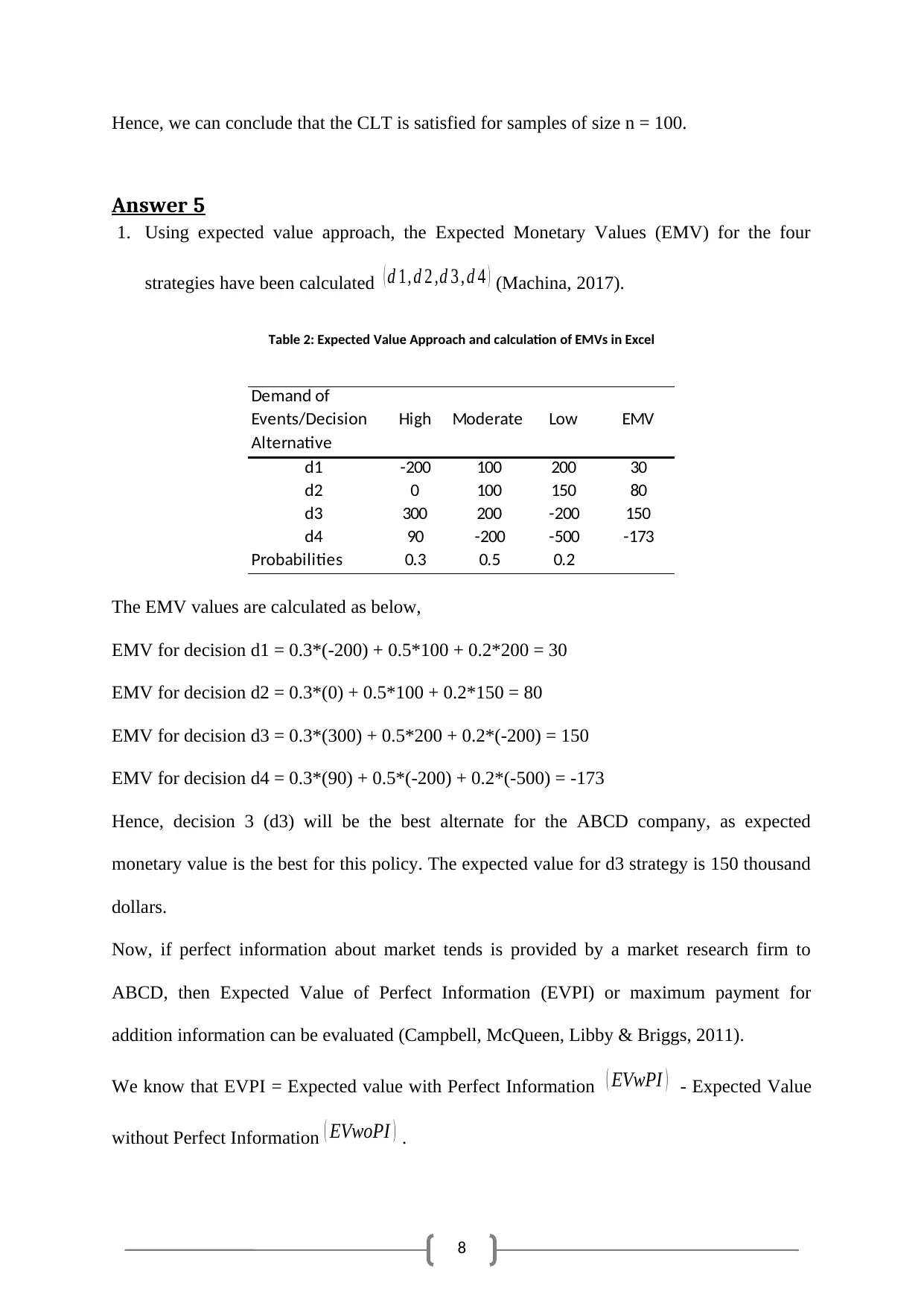
Answer 5
1. Using expected value approach, the Expected Monetary Values (EMV) for the four
strategies have been calculated ( d 1, d 2 ,d 3 , d 4 ) (Machina, 2017).
Table 2: Expected Value Approach and calculation of EMVs in Excel
Demand of
Events/Decision
Alternative
High Moderate Low EMV
d1 -200 100 200 30
d2 0 100 150 80
d3 300 200 -200 150
d4 90 -200 -500 -173
Probabilities 0.3 0.5 0.2
The EMV values are calculated as below,
EMV for decision d1 = 0.3*(-200) + 0.5*100 + 0.2*200 = 30
EMV for decision d2 = 0.3*(0) + 0.5*100 + 0.2*150 = 80
EMV for decision d3 = 0.3*(300) + 0.5*200 + 0.2*(-200) = 150
EMV for decision d4 = 0.3*(90) + 0.5*(-200) + 0.2*(-500) = -173
Hence, decision 3 (d3) will be the best alternate for the ABCD company, as expected
monetary value is the best for this policy. The expected value for d3 strategy is 150 thousand
dollars.
Now, if perfect information about market tends is provided by a market research firm to
ABCD, then Expected Value of Perfect Information (EVPI) or maximum payment for
addition information can be evaluated (Campbell, McQueen, Libby & Briggs, 2011).
We know that EVPI = Expected value with Perfect Information ( EVwPI ) - Expected Value
without Perfect Information ( EVwoPI ) .
Hence, we can conclude that the CLT is satisfied for samples of size n = 100.
Answer 5
1. Using expected value approach, the Expected Monetary Values (EMV) for the four
strategies have been calculated ( d 1, d 2 ,d 3 , d 4 ) (Machina, 2017).
Table 2: Expected Value Approach and calculation of EMVs in Excel
Demand of
Events/Decision
Alternative
High Moderate Low EMV
d1 -200 100 200 30
d2 0 100 150 80
d3 300 200 -200 150
d4 90 -200 -500 -173
Probabilities 0.3 0.5 0.2
The EMV values are calculated as below,
EMV for decision d1 = 0.3*(-200) + 0.5*100 + 0.2*200 = 30
EMV for decision d2 = 0.3*(0) + 0.5*100 + 0.2*150 = 80
EMV for decision d3 = 0.3*(300) + 0.5*200 + 0.2*(-200) = 150
EMV for decision d4 = 0.3*(90) + 0.5*(-200) + 0.2*(-500) = -173
Hence, decision 3 (d3) will be the best alternate for the ABCD company, as expected
monetary value is the best for this policy. The expected value for d3 strategy is 150 thousand
dollars.
Now, if perfect information about market tends is provided by a market research firm to
ABCD, then Expected Value of Perfect Information (EVPI) or maximum payment for
addition information can be evaluated (Campbell, McQueen, Libby & Briggs, 2011).
We know that EVPI = Expected value with Perfect Information ( EVwPI ) - Expected Value
without Perfect Information ( EVwoPI ) .

9
Now ( EVwoPI ) = Maximum EMV = 150 thousand dollars.
The expected value with perfect information is calculated for maximum profits under any
specific market condition.
Hence, ( EVwPI ) = 0.3*300 + 0.5*200 + 0.2*200 = 230 thousand dollars.
So, EVPI = ( EVwPI ) - ( EVwoPI ) =230-150 = 80 thousand dollars. Hence, the value of the
perfect information will be 80 thousand dollars.
⊘ This is a preview!⊘
Do you want full access?
Subscribe today to unlock all pages.
Trusted by 1+ million students worldwide

10
Paraphrase This Document
Need a fresh take? Get an instant paraphrase of this document with our AI Paraphraser
11
References
Campbell, J., McQueen, R., Libby, A., & Briggs, A. (2011). CE1 COST-EFFECTIVENESS
SENSITIVITY ANALYSIS METHODS: A COMPARISON OF ONE-WAY
SENSITIVITY, ANALYSIS OF COVARIANCE, AND EXPECTED VALUE OF
PARTIAL PERFECT INFORMATION. Value In Health, 14(3), A5. doi:
10.1016/j.jval.2011.02.030
Feller, W. (2015). The Fundamental Limit Theorems in Probability. In W. Feller, R. L.
Schilling, Z. Vondraček, & W. A. Woyczyński (Eds.), Selected Papers I (pp. 667–
699). Cham: Springer International Publishing. https://doi.org/10.1007/978-3-319-
16859-3_33
Machina, M. J. (2017). Expected Utility Hypothesis. In The New Palgrave Dictionary of
Economics (pp. 1–12). London: Palgrave Macmillan UK. https://doi.org/10.1057/978-
1-349-95121-5_127-2
Munier, N., Hontoria, E., & Jiménez-Sáez, F. (2019). Linear Programming Fundamentals. In
N. Munier, E. Hontoria, & F. Jiménez-Sáez (Eds.), Strategic Approach in Multi-
Criteria Decision Making: A Practical Guide for Complex Scenarios (pp. 101–116).
Cham: Springer International Publishing. https://doi.org/10.1007/978-3-030-02726-1_6
Rani Das, K. (2016). A Brief Review of Tests for Normality. American Journal Of
Theoretical And Applied Statistics, 5(1), 5. https://doi: 10.11648/j.ajtas.20160501.12
Vanderbei, R. J. (2014). The Simplex Method. In R. J. Vanderbei (Ed.), Linear
Programming: Foundations and Extensions (pp. 11–23). Boston, MA: Springer US.
https://doi.org/10.1007/978-1-4614-7630-6_2
Wulan, E. R., Ramdhani, M. A., & Indriani. (2018). Determine the Optimal Solution for
Linear Programming with Interval Coefficients. IOP Conference Series: Materials

12
Science and Engineering, 288, 012061.
https://doi.org/10.1088/1757-899X/288/1/012061
Science and Engineering, 288, 012061.
https://doi.org/10.1088/1757-899X/288/1/012061
⊘ This is a preview!⊘
Do you want full access?
Subscribe today to unlock all pages.
Trusted by 1+ million students worldwide
1 out of 12

Your All-in-One AI-Powered Toolkit for Academic Success.
+13062052269
info@desklib.com
Available 24*7 on WhatsApp / Email
![[object Object]](/_next/static/media/star-bottom.7253800d.svg)
Unlock your academic potential
Copyright © 2020–2026 A2Z Services. All Rights Reserved. Developed and managed by ZUCOL.