Linear Programming and Forecasting

This study material discusses the concepts and applications of linear programming and forecasting. It includes case studies on optimizing loan plans and forecasting sales revenue. The material also provides sensitivity reports and analysis of different forecasting methods.

Running head: LINEAR PROGRAMMING AND FORECASTING
Linear Programming and Forecasting
Name of the Student:
Name of the University:
Author’s Note:

1LINEAR PROGRAMMING AND FORECASTING
Table of Contents
Introduction:....................................................................................................................................2
Answer 1.A:.....................................................................................................................................2
Answer 1.B.1...................................................................................................................................4
Answer 1.B.2...................................................................................................................................5
Answer 1.B.3...................................................................................................................................7
Answer 3.A......................................................................................................................................8
Answer 3.B......................................................................................................................................9
Conclusion.....................................................................................................................................10
Reference:......................................................................................................................................11

2LINEAR PROGRAMMING AND FORECASTING
Introduction:
Linear programming is extensively utilized in mathematical modelling and techniques
which is applied to obtain the most favourable results or solutions with respect to the given
various constraint that are expressed in a linear relationship (Dantzig, 2016). Forecasting is
important to make plans for effective operations. Planning is not possible without prediction of
future and forecasting is an analysis of the future (De Giorgi, Congedo, & Malvoni, 2014).
Here two case studies are where linear programming and forecasting is widely applied.
The linear programming model have to derive the optimum loan plan that minimises the total
amount of loan interest for Mathew and the forecast of monthly paid lettings needs to be done for
China-based boutique. The results of these two case studies are discussed below (Vanderbei,
2015).
Answer 1.A:
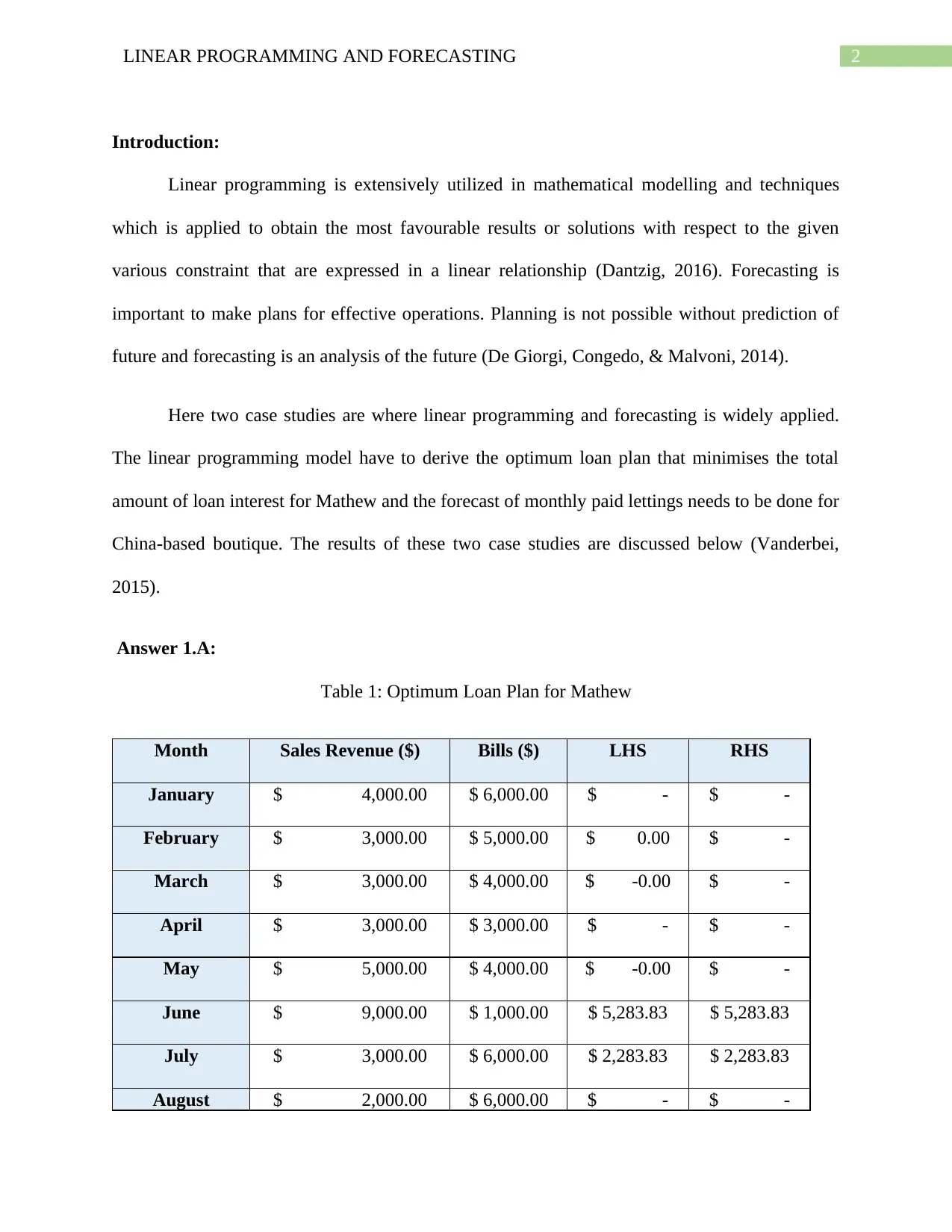
Table 1: Optimum Loan Plan for Mathew
Month Sales Revenue ($) Bills ($) LHS RHS
January $ 4,000.00 $ 6,000.00 $ - $ -
February $ 3,000.00 $ 5,000.00 $ 0.00 $ -
March $ 3,000.00 $ 4,000.00 $ -0.00 $ -
April $ 3,000.00 $ 3,000.00 $ - $ -
May $ 5,000.00 $ 4,000.00 $ -0.00 $ -
June $ 9,000.00 $ 1,000.00 $ 5,283.83 $ 5,283.83
July $ 3,000.00 $ 6,000.00 $ 2,283.83 $ 2,283.83
August $ 2,000.00 $ 6,000.00 $ - $ -

3LINEAR PROGRAMMING AND FORECASTING
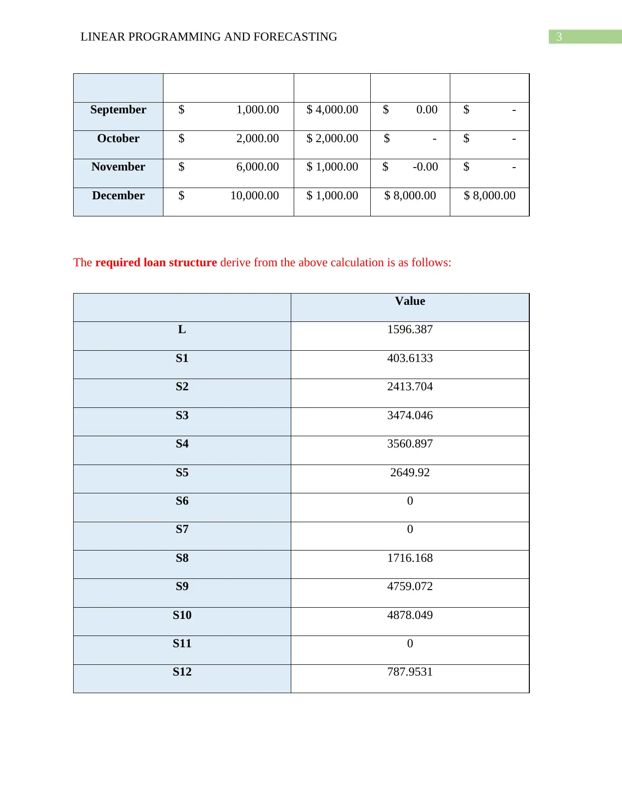
September $ 1,000.00 $ 4,000.00 $ 0.00 $ -
October $ 2,000.00 $ 2,000.00 $ - $ -
November $ 6,000.00 $ 1,000.00 $ -0.00 $ -
December $ 10,000.00 $ 1,000.00 $ 8,000.00 $ 8,000.00
The required loan structure derive from the above calculation is as follows:
Value
L 1596.387
S1 403.6133
S2 2413.704
S3 3474.046
S4 3560.897
S5 2649.92
S6 0
S7 0
S8 1716.168
S9 4759.072
S10 4878.049
S11 0
S12 787.9531

4LINEAR PROGRAMMING AND FORECASTING
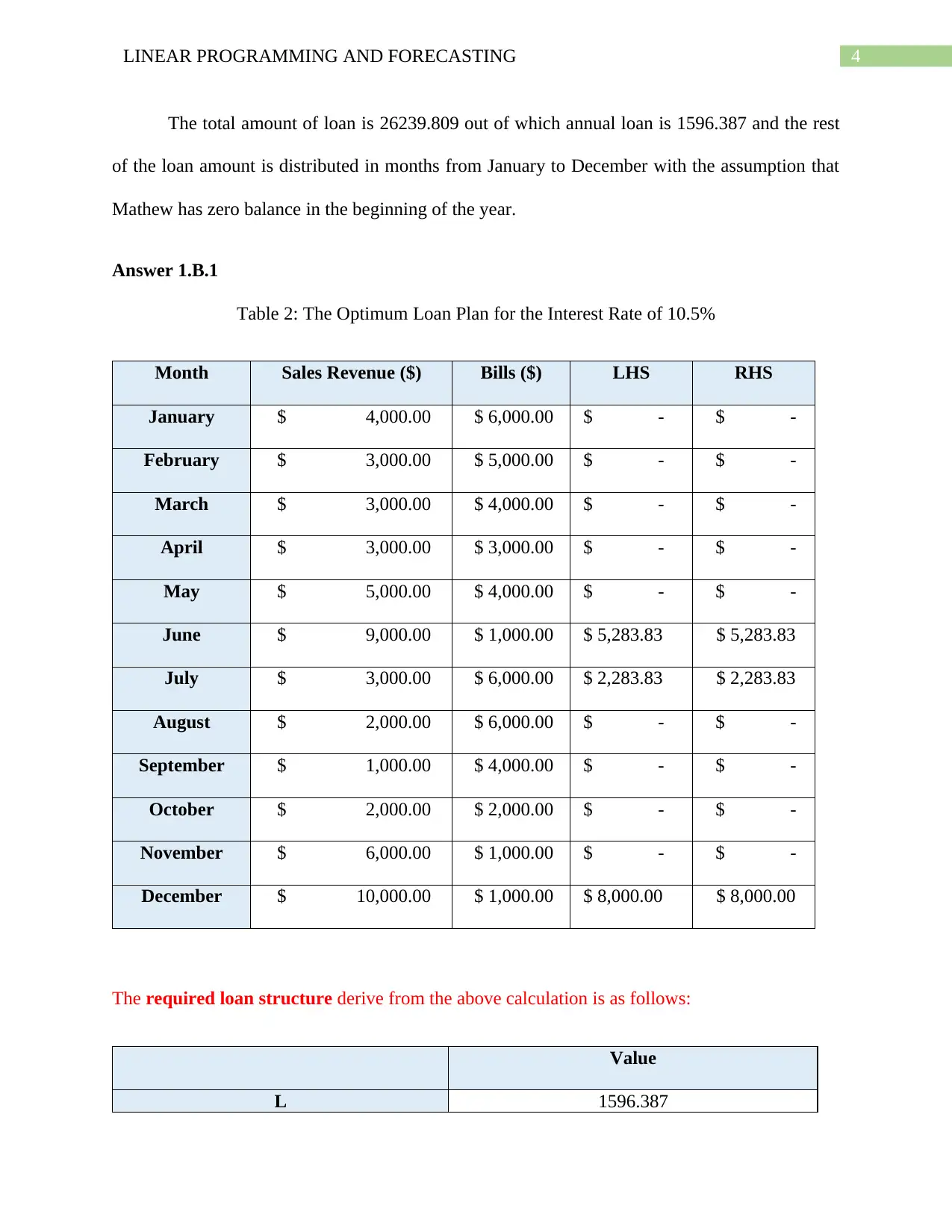
The total amount of loan is 26239.809 out of which annual loan is 1596.387 and the rest
of the loan amount is distributed in months from January to December with the assumption that
Mathew has zero balance in the beginning of the year.
Answer 1.B.1
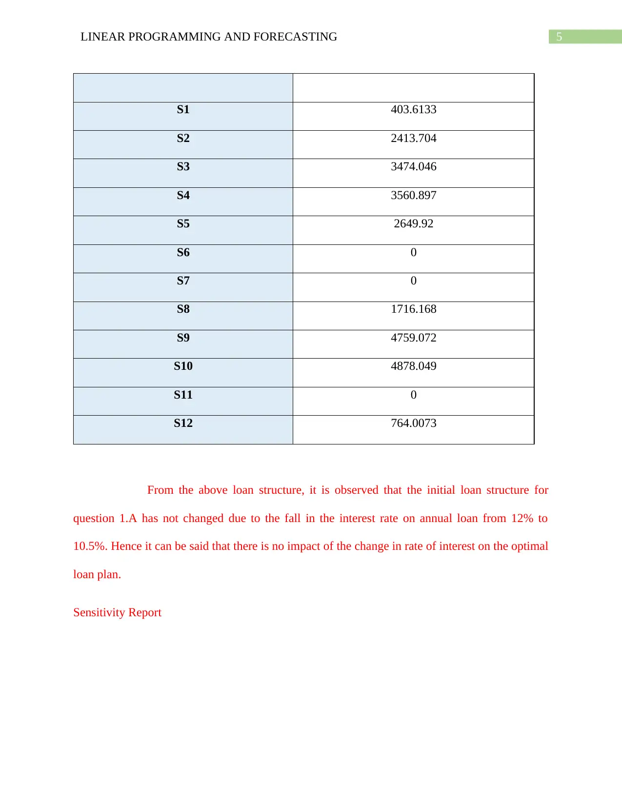
Table 2: The Optimum Loan Plan for the Interest Rate of 10.5%
Month Sales Revenue ($) Bills ($) LHS RHS
January $ 4,000.00 $ 6,000.00 $ - $ -
February $ 3,000.00 $ 5,000.00 $ - $ -
March $ 3,000.00 $ 4,000.00 $ - $ -
April $ 3,000.00 $ 3,000.00 $ - $ -
May $ 5,000.00 $ 4,000.00 $ - $ -
June $ 9,000.00 $ 1,000.00 $ 5,283.83 $ 5,283.83
July $ 3,000.00 $ 6,000.00 $ 2,283.83 $ 2,283.83
August $ 2,000.00 $ 6,000.00 $ - $ -
September $ 1,000.00 $ 4,000.00 $ - $ -
October $ 2,000.00 $ 2,000.00 $ - $ -
November $ 6,000.00 $ 1,000.00 $ - $ -
December $ 10,000.00 $ 1,000.00 $ 8,000.00 $ 8,000.00
The required loan structure derive from the above calculation is as follows:
Value
L 1596.387

5LINEAR PROGRAMMING AND FORECASTING
S1 403.6133
S2 2413.704
S3 3474.046
S4 3560.897
S5 2649.92
S6 0
S7 0
S8 1716.168
S9 4759.072
S10 4878.049
S11 0
S12 764.0073
From the above loan structure, it is observed that the initial loan structure for
question 1.A has not changed due to the fall in the interest rate on annual loan from 12% to
10.5%. Hence it can be said that there is no impact of the change in rate of interest on the optimal
loan plan.
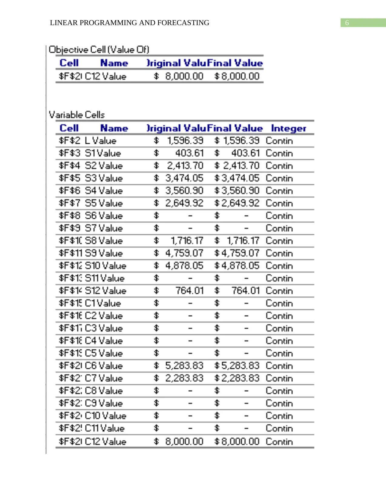
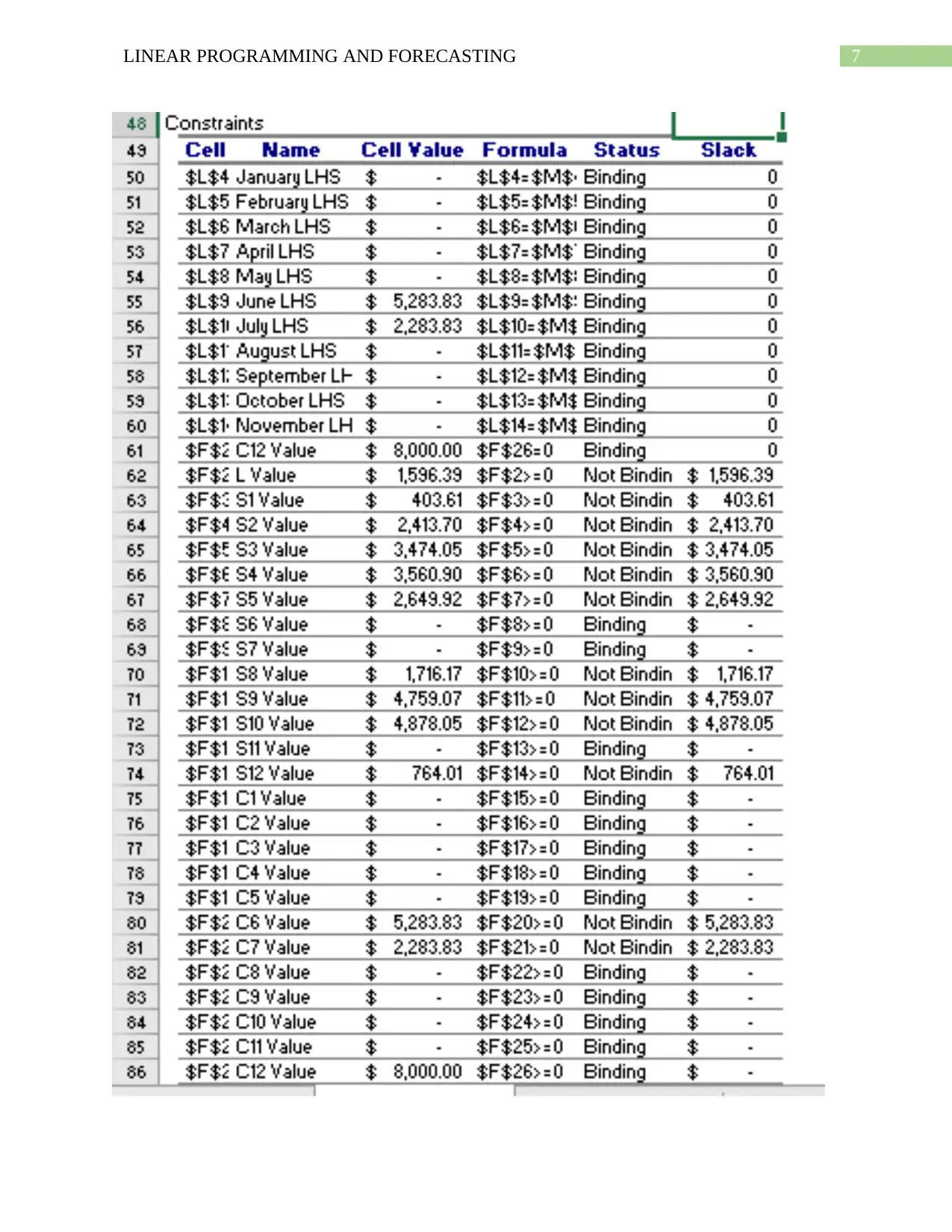
Sensitivity Report

6LINEAR PROGRAMMING AND FORECASTING

7LINEAR PROGRAMMING AND FORECASTING

8LINEAR PROGRAMMING AND FORECASTING
Answer 1.B.2
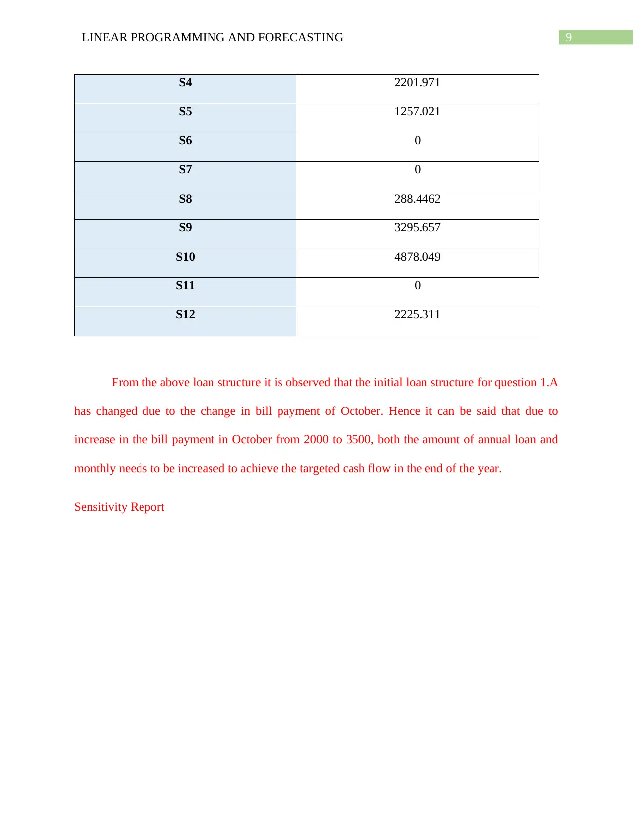
Table 3: Loan Plan When the Bill to Pay of October is $3500
Month Sales Revenue ($) Bills ($) LHS RHS
January $ 4,000.00 $ 6,000.00 $ 879.74 $ 879.74
February $ 3,000.00 $ 5,000.00 $ - $ -
March $ 3,000.00 $ 4,000.00 $ -0.00 $ -
April $ 3,000.00 $ 3,000.00 $ - $ -
May $ 5,000.00 $ 4,000.00 $ -0.00 $ -
June $ 9,000.00 $ 1,000.00 $ 6,711.55 $ 6,711.55
July $ 3,000.00 $ 6,000.00 $ 3,711.55 $ 3,711.55
August $ 2,000.00 $ 6,000.00 $ - $ -
September $ 1,000.00 $ 4,000.00 $ 0.00 $ -
October $ 2,000.00 $ 3,500.00 $ 0.00 $ -
November $ 6,000.00 $ 1,000.00 $ -0.00 $ -
December $ 10,000.00 $ 1,000.00 $ 8,000.00 $ 8,000.00
The required loan structure derive from the above calculation is as follows:
Value
L 2879.742
S1 0
S2 1120.258
S3 2148.265

9LINEAR PROGRAMMING AND FORECASTING
S4 2201.971
S5 1257.021
S6 0
S7 0
S8 288.4462
S9 3295.657
S10 4878.049
S11 0
S12 2225.311
From the above loan structure it is observed that the initial loan structure for question 1.A
has changed due to the change in bill payment of October. Hence it can be said that due to
increase in the bill payment in October from 2000 to 3500, both the amount of annual loan and
monthly needs to be increased to achieve the targeted cash flow in the end of the year.
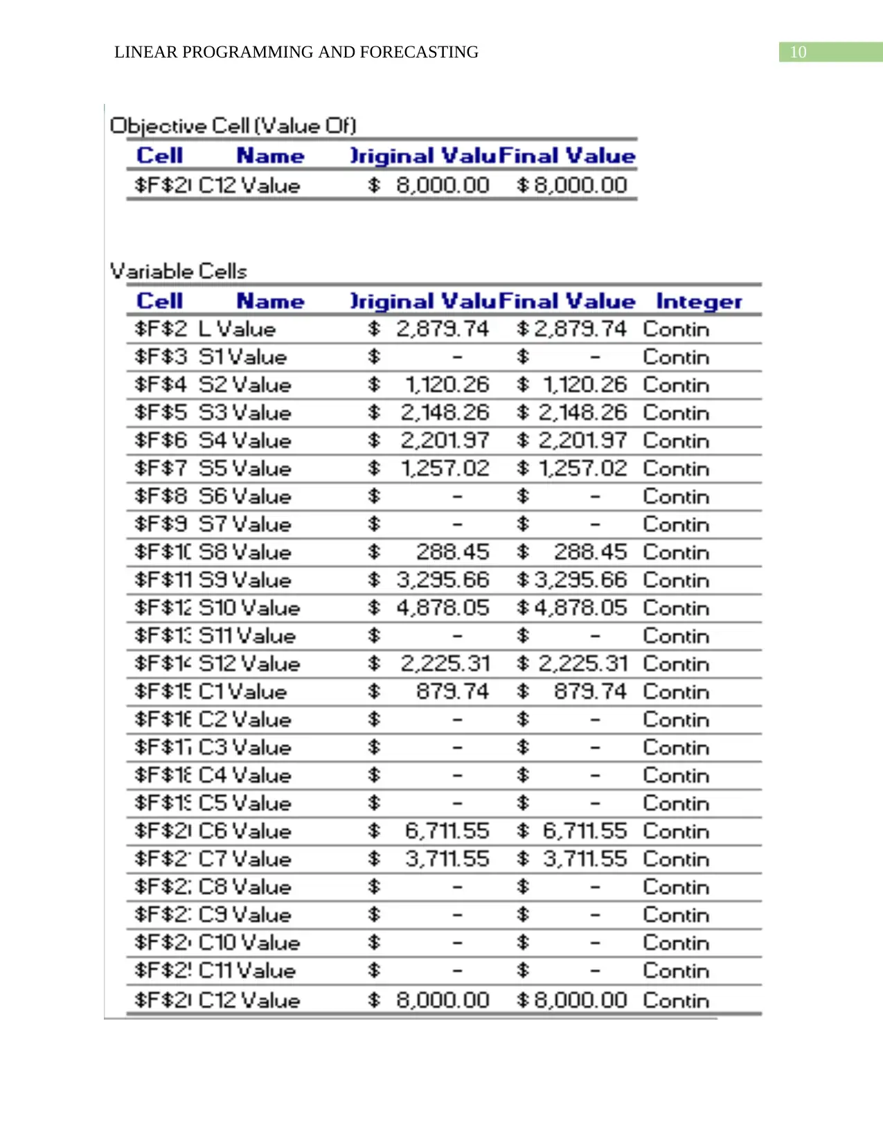
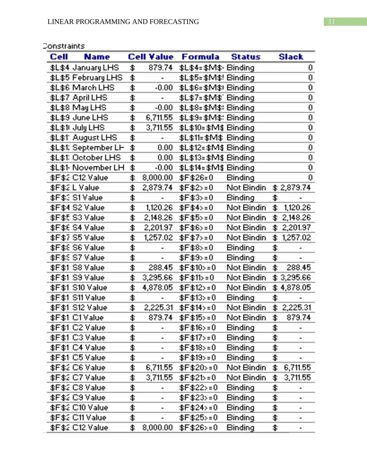
Sensitivity Report

10LINEAR PROGRAMMING AND FORECASTING

11LINEAR PROGRAMMING AND FORECASTING

12LINEAR PROGRAMMING AND FORECASTING
Answer 1.B.3
Table 4: Loan Plan for the Revised Forecast of Sales Amount of September
Month Sales Revenue ($) Bills ($) LHS RHS
January $ 4,000.00 $ 6,000.00 $ - $ -
February $ 3,000.00 $ 5,000.00 $ 0.00 $ -
March $ 3,000.00 $ 4,000.00 $ -0.00 $ -
April $ 3,000.00 $ 3,000.00 $ - $ -
May $ 5,000.00 $ 4,000.00 $ -0.00 $ -
June $ 9,000.00 $ 1,000.00 $ 5,248.14 $ 5,248.14
July $ 3,000.00 $ 6,000.00 $ 2,248.14 $ 2,248.14
August $ 2,000.00 $ 6,000.00 $ - $ -
September $ 2,500.00 $ 4,000.00 $ 0.00 $ -
October $ 2,000.00 $ 3,500.00 $ 0.00 $ -
November $ 6,000.00 $ 1,000.00 $ -0.00 $ -
December $ 10,000.00 $ 1,000.00 $ 8,000.00 $ 8,000.00
The required loan structure derive from the above calculation is as follows:
Value
L 1564.839
S1 435.1607
S2 2446.04
S3 3507.191

13LINEAR PROGRAMMING AND FORECASTING
S4 3594.871
S5 2684.742
S6 0
S7 0
S8 1751.861
S9 3295.657
S10 4878.049
S11 0
S12 752.62
The above loan structure, it is observed that the initial loan structure for question
1.A has changed due to the change in the forecast of sales in September. Due to increase in the
forecast of sales in September from 1000 to 2500, both the amount of annual loan and monthly
loan needs to be decreased slightly to achieve the targeted cash flow in the end of the year.
Sensitivity Report

14LINEAR PROGRAMMING AND FORECASTING

15LINEAR PROGRAMMING AND FORECASTING

16LINEAR PROGRAMMING AND FORECASTING
Answer 3.A
Table 5: MAD and MAPE for the Forecasting Methods.
Moving Average Exponential Regression
Multiplicativ
e Forecast
MAD 51067.76 45476.78 56921.92 45887.79
MAPE 5.03% 4.42% 6.09% 5.15%
To determine which method needs to be applied in this case, the MAD and MAPE are
calculated for each method. The lowest value of MAD and MAPE is for the exponential method
that means this method will give the best forecast for the paid lettings (Barnes et al. 2016).
Table 6: SE for the Forecast of Each Year
Year Mean SE
2007 45224.41 10141.9
2008 39044.59 8810.272
2009 44217.93 9285.527
2010 48839.23 11320.32
2011 39053.87 10281.76
2012 33458.27 7953.273
2013 46723.33 9408.934
2014 44277.86 10364.3
2015 69733.89 11415.54
2016 51316.51 18728.15

17LINEAR PROGRAMMING AND FORECASTING
2017 45320.62 13457.65
2018 31502.83 17874.52
The above tables contains the SE of each year’s forecast to determine which time period
of data is relevant for the forecasting. The SE is too high for the year 2016, 2017 and 2018,
therefore, these years are irrelevant for the forecasting and the rest means 2007, 2008, 2009,
2010, 2011, 2012, 2013, 2014 and 2015 are relevant years for the forecasting (Trzaskuś-Żak,
2018).
Answer 3.B
The exponential forecasting method is applied to forecast the paid lettings of the year
2019 which takes the dumping value of 0.5 which shows the lowest MAD, MSE and MAPE. The
below table shows the MAD, MSE and MAPE value for the forecast (Mamula, 2015).
Table 7: MAD, MSE and MAPE for the Dumping Value 0.5
Dumping MAD MSE MAPE
α=0.5 45476.78 59799.55 4.42%
The monthly paid lettings for the year 2019 is 1487106 for all the months over the year.
The limitation of the exponential forecasting is that the forecast value is constant for all the
variables (Bergmeir, Hyndman & Benítez 2016).

18LINEAR PROGRAMMING AND FORECASTING
Conclusion
The linear programming solutions can easily calculate the optimum values of dynamic
problem. In the above discussion Mathew got the optimum level of loan plan. The forecasting for
the chian-based restaurant and boutique has the predicted value of the paid lettings for the year
2019 (Anderson et al. 2018). With this it can plan for the business.

19LINEAR PROGRAMMING AND FORECASTING
Reference:
Anderson, D. R., Sweeney, D. J., Williams, T. A., Camm, J. D., & Cochran, J. J. (2018). An
introduction to management science: quantitative approach. Cengage learning.
Barnes, G., Leka, K. D., Schrijver, C. J., Colak, T., Qahwaji, R., Ashamari, O. W., ... & Higgins,
P. A. (2016). A Comparison of flare forecasting methods. I. Results from the “all-clear”
workshop. The Astrophysical Journal, 829(2), 89.
Bergmeir, C., Hyndman, R. J., & Benítez, J. M. (2016). Bagging exponential smoothing methods
using STL decomposition and Box–Cox transformation. International journal of
forecasting, 32(2), 303-312.
Dantzig, G. (2016). Linear programming and extensions. Princeton university press.
De Giorgi, M. G., Congedo, P. M., & Malvoni, M. (2014). Photovoltaic power forecasting using
statistical methods: impact of weather data. IET Science, Measurement &
Technology, 8(3), 90-97.
Mamula, M. (2015). Modelling and forecasting international tourism demand-evaluation of
forecasting performance. International Journal of Business Administration, 6(3), 102.
Trzaskuś-Żak, B. (2018). Implementation of the Exponential Smoothing Method for Forecasting
of the Sales Volume of an Opencast Mine of Rock and Raw Materials. Inżynieria
Mineralna, 20.
Vanderbei, R. J. (2015). Linear programming. Heidelberg: Springer.