Linear Programming Model Building and Decision Trees in Logistics and Supply Chain Management

This article discusses capacity decision making, ordering approaches, and line balancing in logistics and supply chain management. It covers topics such as linear programming model building and decision trees to help optimize business decisions. The article provides examples and models to illustrate these concepts.

SCHOOL OF MANAGEMENT
MSC LOGISTICS AND SUPPLY CHAIN MANAGEMENT
MSC PROCUREMENT AND SUPPLY CHAIN MANAGEMENT

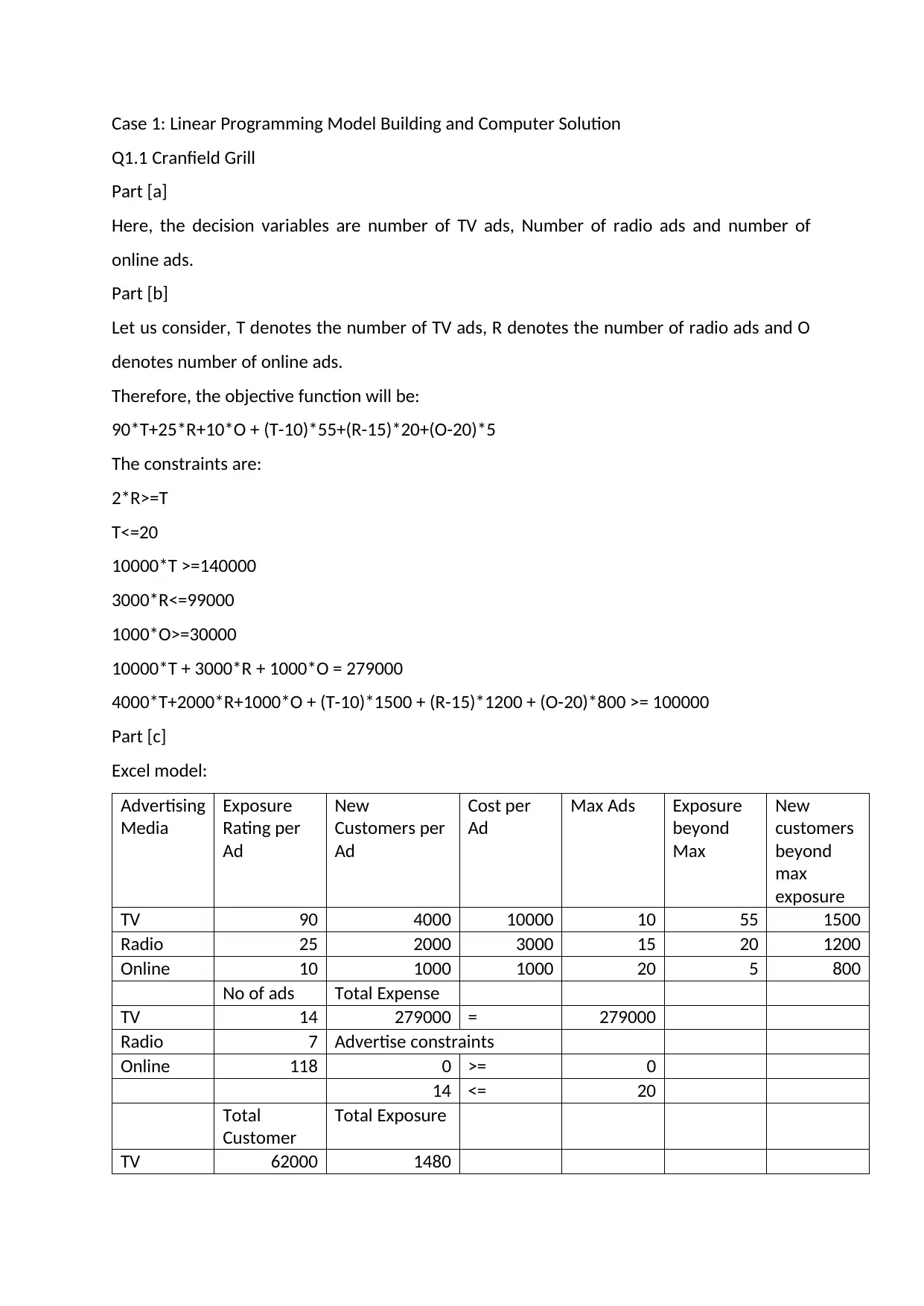
Case 1: Linear Programming Model Building and Computer Solution
Q1.1 Cranfield Grill
Part [a]
Here, the decision variables are number of TV ads, Number of radio ads and number of
online ads.
Part [b]
Let us consider, T denotes the number of TV ads, R denotes the number of radio ads and O
denotes number of online ads.
Therefore, the objective function will be:
90*T+25*R+10*O + (T-10)*55+(R-15)*20+(O-20)*5
The constraints are:
2*R>=T
T<=20
10000*T >=140000
3000*R<=99000
1000*O>=30000
10000*T + 3000*R + 1000*O = 279000
4000*T+2000*R+1000*O + (T-10)*1500 + (R-15)*1200 + (O-20)*800 >= 100000
Part [c]
Excel model:
Advertising
Media
Exposure
Rating per
Ad
New
Customers per
Ad
Cost per
Ad
Max Ads Exposure
beyond
Max
New
customers
beyond
max
exposure
TV 90 4000 10000 10 55 1500
Radio 25 2000 3000 15 20 1200
Online 10 1000 1000 20 5 800
No of ads Total Expense
TV 14 279000 = 279000
Radio 7 Advertise constraints
Online 118 0 >= 0
14 <= 20
Total
Customer
Total Exposure
TV 62000 1480

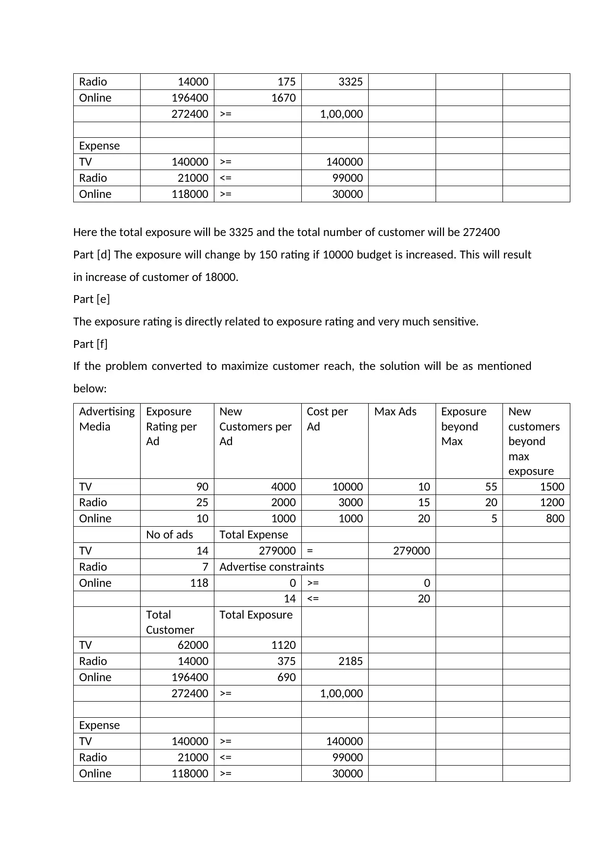
Radio 14000 175 3325
Online 196400 1670
272400 >= 1,00,000
Expense
TV 140000 >= 140000
Radio 21000 <= 99000
Online 118000 >= 30000
Here the total exposure will be 3325 and the total number of customer will be 272400
Part [d] The exposure will change by 150 rating if 10000 budget is increased. This will result
in increase of customer of 18000.
Part [e]
The exposure rating is directly related to exposure rating and very much sensitive.
Part [f]
If the problem converted to maximize customer reach, the solution will be as mentioned
below:
Advertising
Media
Exposure
Rating per
Ad
New
Customers per
Ad
Cost per
Ad
Max Ads Exposure
beyond
Max
New
customers
beyond
max
exposure
TV 90 4000 10000 10 55 1500
Radio 25 2000 3000 15 20 1200
Online 10 1000 1000 20 5 800
No of ads Total Expense
TV 14 279000 = 279000
Radio 7 Advertise constraints
Online 118 0 >= 0
14 <= 20
Total
Customer
Total Exposure
TV 62000 1120
Radio 14000 375 2185
Online 196400 690
272400 >= 1,00,000
Expense
TV 140000 >= 140000
Radio 21000 <= 99000
Online 118000 >= 30000

It means, maximum 272400 people can be reached.
Part [g]
Maximizing customer reach will make much more sense than maximizing exposure, as this
will directly improve the sales volume, when there is a chance that the exposure will not be
converted to sales to some extent.
Q1.2 Cranfield Materials
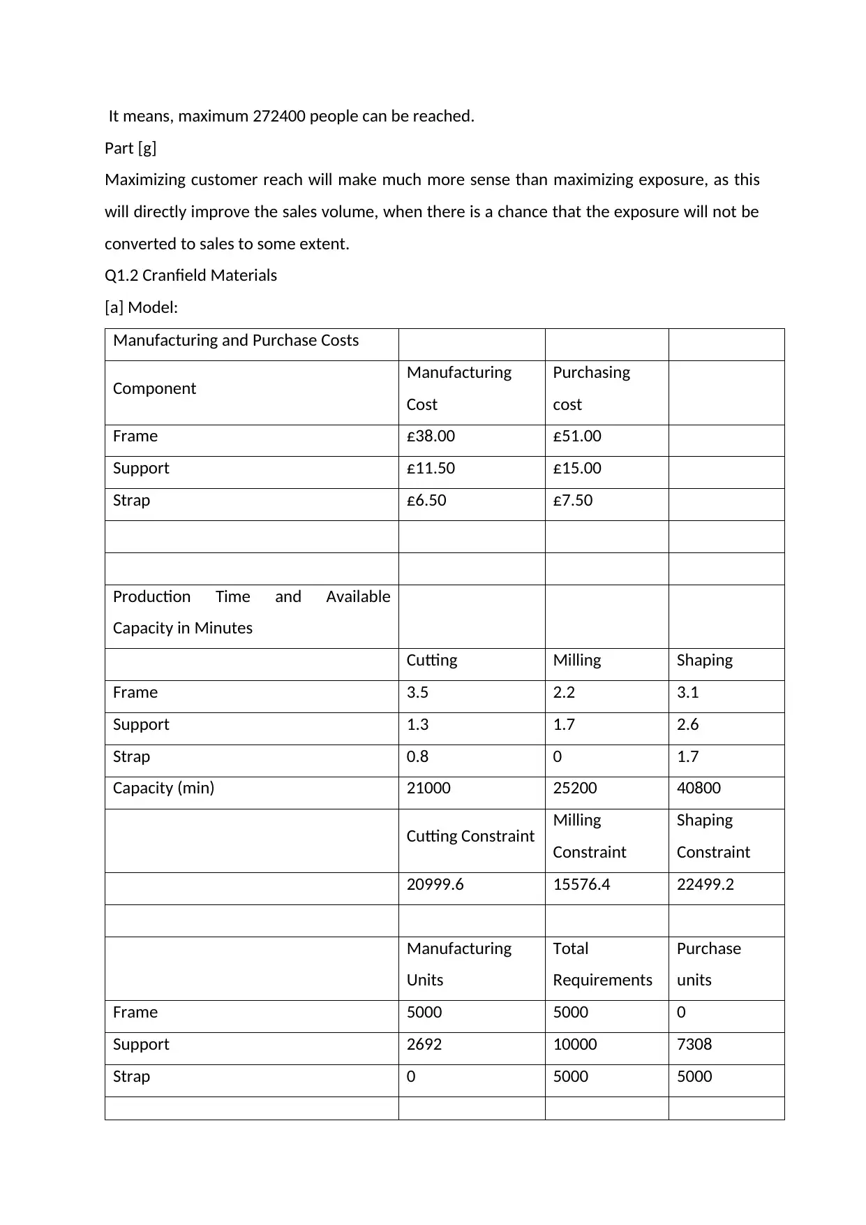
[a] Model:
Manufacturing and Purchase Costs
Component Manufacturing
Cost
Purchasing
cost
Frame £38.00 £51.00
Support £11.50 £15.00
Strap £6.50 £7.50
Production Time and Available
Capacity in Minutes
Cutting Milling Shaping
Frame 3.5 2.2 3.1
Support 1.3 1.7 2.6
Strap 0.8 0 1.7
Capacity (min) 21000 25200 40800
Cutting Constraint Milling
Constraint
Shaping
Constraint
20999.6 15576.4 22499.2
Manufacturing
Units
Total
Requirements
Purchase
units
Frame 5000 5000 0
Support 2692 10000 7308
Strap 0 5000 5000

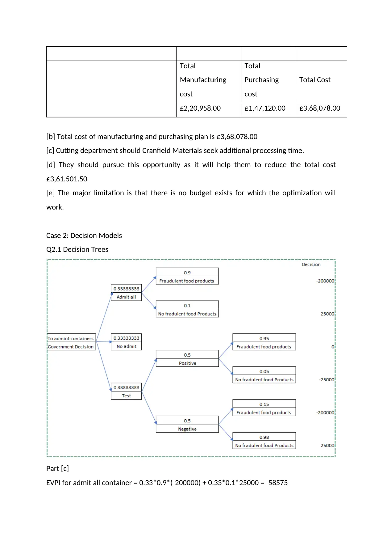
Total
Manufacturing
cost
Total
Purchasing
cost
Total Cost
£2,20,958.00 £1,47,120.00 £3,68,078.00
[b] Total cost of manufacturing and purchasing plan is £3,68,078.00
[c] Cutting department should Cranfield Materials seek additional processing time.
[d] They should pursue this opportunity as it will help them to reduce the total cost
£3,61,501.50
[e] The major limitation is that there is no budget exists for which the optimization will
work.
Case 2: Decision Models
Q2.1 Decision Trees
Part [c]
EVPI for admit all container = 0.33*0.9*(-200000) + 0.33*0.1*25000 = -58575

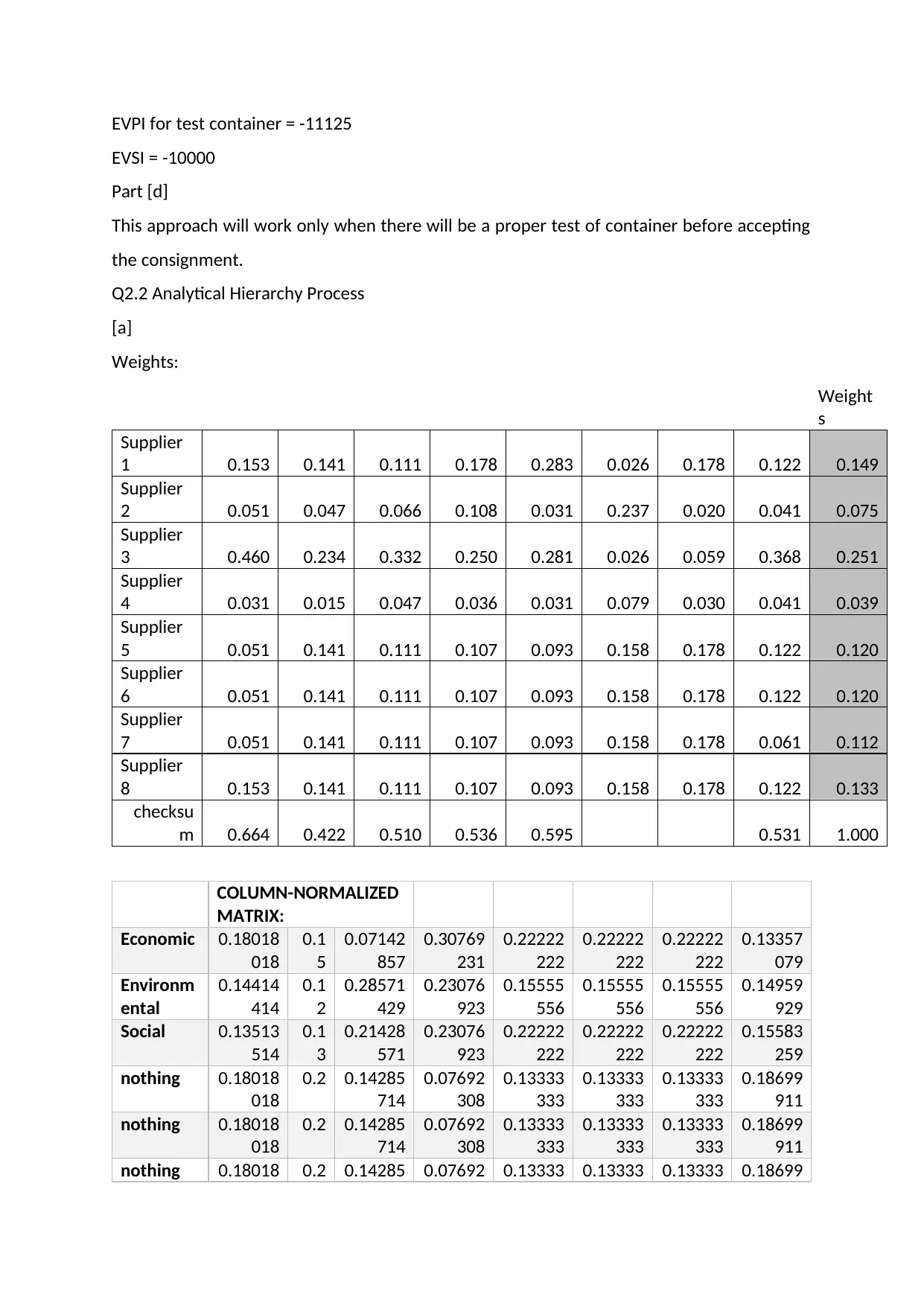
EVPI for test container = -11125
EVSI = -10000
Part [d]
This approach will work only when there will be a proper test of container before accepting
the consignment.
Q2.2 Analytical Hierarchy Process
[a]
Weights:
Weight
s
Supplier
1 0.153 0.141 0.111 0.178 0.283 0.026 0.178 0.122 0.149
Supplier
2 0.051 0.047 0.066 0.108 0.031 0.237 0.020 0.041 0.075
Supplier
3 0.460 0.234 0.332 0.250 0.281 0.026 0.059 0.368 0.251
Supplier
4 0.031 0.015 0.047 0.036 0.031 0.079 0.030 0.041 0.039
Supplier
5 0.051 0.141 0.111 0.107 0.093 0.158 0.178 0.122 0.120
Supplier
6 0.051 0.141 0.111 0.107 0.093 0.158 0.178 0.122 0.120
Supplier
7 0.051 0.141 0.111 0.107 0.093 0.158 0.178 0.061 0.112
Supplier
8 0.153 0.141 0.111 0.107 0.093 0.158 0.178 0.122 0.133
checksu
m 0.664 0.422 0.510 0.536 0.595 0.531 1.000
COLUMN-NORMALIZED
MATRIX:
Economic 0.18018
018
0.1
5
0.07142
857
0.30769
231
0.22222
222
0.22222
222
0.22222
222
0.13357
079
Environm
ental
0.14414
414
0.1
2
0.28571
429
0.23076
923
0.15555
556
0.15555
556
0.15555
556
0.14959
929
Social 0.13513
514
0.1
3
0.21428
571
0.23076
923
0.22222
222
0.22222
222
0.22222
222
0.15583
259
nothing 0.18018
018
0.2 0.14285
714
0.07692
308
0.13333
333
0.13333
333
0.13333
333
0.18699
911
nothing 0.18018
018
0.2 0.14285
714
0.07692
308
0.13333
333
0.13333
333
0.13333
333
0.18699
911
nothing 0.18018 0.2 0.14285 0.07692 0.13333 0.13333 0.13333 0.18699

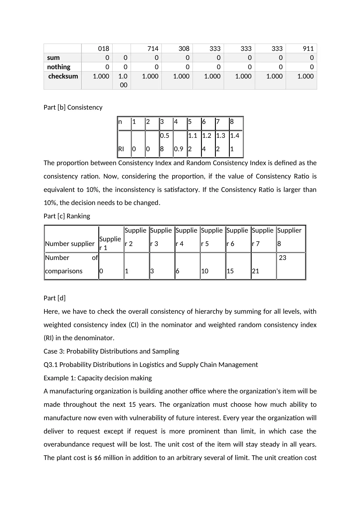
018 714 308 333 333 333 911
sum 0 0 0 0 0 0 0 0
nothing 0 0 0 0 0 0 0 0
checksum 1.000 1.0
00
1.000 1.000 1.000 1.000 1.000 1.000
Part [b] Consistency
n 1 2 3 4 5 6 7 8
RI 0 0
0.5
8 0.9
1.1
2
1.2
4
1.3
2
1.4
1
The proportion between Consistency Index and Random Consistency Index is defined as the
consistency ration. Now, considering the proportion, if the value of Consistency Ratio is
equivalent to 10%, the inconsistency is satisfactory. If the Consistency Ratio is larger than
10%, the decision needs to be changed.
Part [c] Ranking
Number supplier Supplie
r 1
Supplie
r 2
Supplie
r 3
Supplie
r 4
Supplie
r 5
Supplie
r 6
Supplie
r 7
Supplier
8
Number of
comparisons 0 1 3 6 10 15 21
23
Part [d]
Here, we have to check the overall consistency of hierarchy by summing for all levels, with
weighted consistency index (CI) in the nominator and weighted random consistency index
(RI) in the denominator.
Case 3: Probability Distributions and Sampling
Q3.1 Probability Distributions in Logistics and Supply Chain Management
Example 1: Capacity decision making
A manufacturing organization is building another office where the organization's item will be
made throughout the next 15 years. The organization must choose how much ability to
manufacture now even with vulnerability of future interest. Every year the organization will
deliver to request except if request is more prominent than limit, in which case the
overabundance request will be lost. The unit cost of the item will stay steady in all years.
The plant cost is $6 million in addition to an arbitrary several of limit. The unit creation cost

is a directly diminishing capacity limit with an arbitrary capture. Additionally, the unit
working expense is irregular. The model expect that every one of these unit costs stays
steady through time, yet it could be adjusted effectively to give them a chance to change
through time.
Example 2: Ordering approaches
An organization faces inconsistent requests for an expensive item. The week by week
request conveyance is discrete. The mean is around 2 every week. The organization
arranges the item from a provider, and the lead time from when a request is put until the
point that it arrives is similarly prone to be 2 or 3 weeks. The organization needs a
requesting approach that keeps normal stock low yet in addition keeps stock-outs low.
The conventional requesting strategy is described by two numbers, a trigger and a request
amount. At the point when on-hand stock falls to the specific benchmark or beneath, and
there is no structure presently being sent, an order for the request amount is set. An
elective requesting arrangement that foresees run of the mill request may be better. With
this approach, the organization has a standard week after week demand of a given size. For
instance, with mean interest around 2 every week, it bodes well that the organization may
arrange 2 every week, despite the fact that the model treats this amount as a choice
variable. Because of arbitrariness sought after, in any case, this standard request size may
prompt excessively or too little stock. Along these lines, the strategy has two triggers and
two other request amounts. On the off chance that stock is at or over the primary trigger,
the week after week arrange is for a littler request amount. In the event that stock is at or
beneath the second trigger, the week by week arrange is for a bigger request amount. So
this "expectant" arrangement is portrayed by five choice factors.
Example 3: Line Balancing
This is a rearranged model of a 5-arrange fabricating process. Each stage has various
indistinguishable machines, and each machine can create an irregular number of things in a
settled day and age. Each stage encourages the following stage. Stage 1 sends its finished
things to organize 2, arrange 2 sends its finished things to organize 3, etc. Notwithstanding,
any phase from stage 2 on can create just the same number of things as it gets, even it can
possibly deliver more. In this way, there is a motivation to adjust the stages with the goal
that their generation rates are comparable. All the more explicitly, the issue is to decide the

quantity of machines at each phase to boost mean benefit, which is the income from
moving all things created amid the period less the working expenses of the machines.
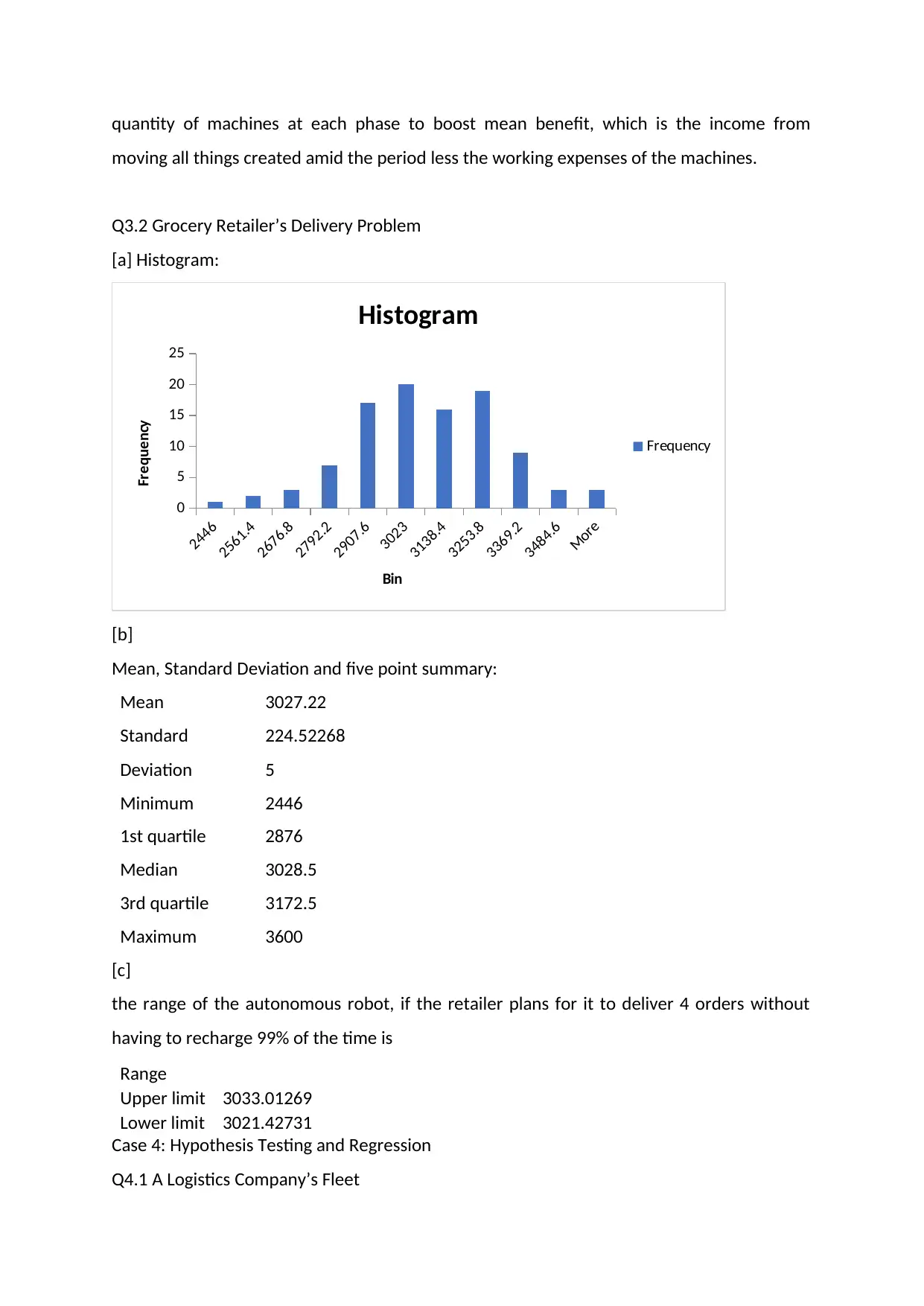
Q3.2 Grocery Retailer’s Delivery Problem
[a] Histogram:
2446
2561.4
2676.8
2792.2
2907.6
3023
3138.4
3253.8
3369.2
3484.6
More
0
5
10
15
20
25
Histogram
Frequency
Bin
Frequency
[b]
Mean, Standard Deviation and five point summary:
Mean 3027.22
Standard
Deviation
224.52268
5
Minimum 2446
1st quartile 2876
Median 3028.5
3rd quartile 3172.5
Maximum 3600
[c]
the range of the autonomous robot, if the retailer plans for it to deliver 4 orders without
having to recharge 99% of the time is
Range
Upper limit 3033.01269
Lower limit 3021.42731
Case 4: Hypothesis Testing and Regression
Q4.1 A Logistics Company’s Fleet

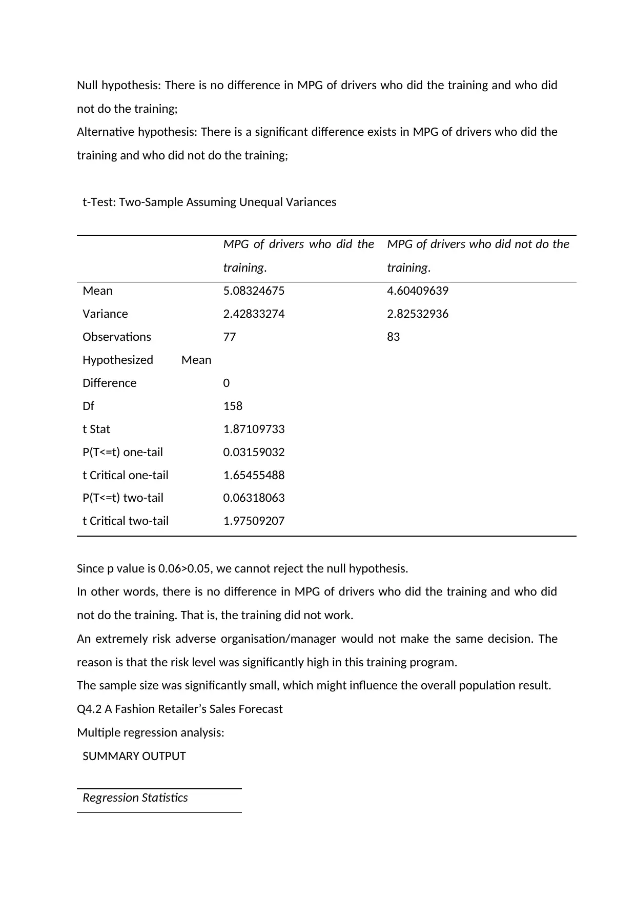
Null hypothesis: There is no difference in MPG of drivers who did the training and who did
not do the training;
Alternative hypothesis: There is a significant difference exists in MPG of drivers who did the
training and who did not do the training;
t-Test: Two-Sample Assuming Unequal Variances
MPG of drivers who did the
training.
MPG of drivers who did not do the
training.
Mean 5.08324675 4.60409639
Variance 2.42833274 2.82532936
Observations 77 83
Hypothesized Mean
Difference 0
Df 158
t Stat 1.87109733
P(T<=t) one-tail 0.03159032
t Critical one-tail 1.65455488
P(T<=t) two-tail 0.06318063
t Critical two-tail 1.97509207
Since p value is 0.06>0.05, we cannot reject the null hypothesis.
In other words, there is no difference in MPG of drivers who did the training and who did
not do the training. That is, the training did not work.
An extremely risk adverse organisation/manager would not make the same decision. The
reason is that the risk level was significantly high in this training program.
The sample size was significantly small, which might influence the overall population result.
Q4.2 A Fashion Retailer’s Sales Forecast
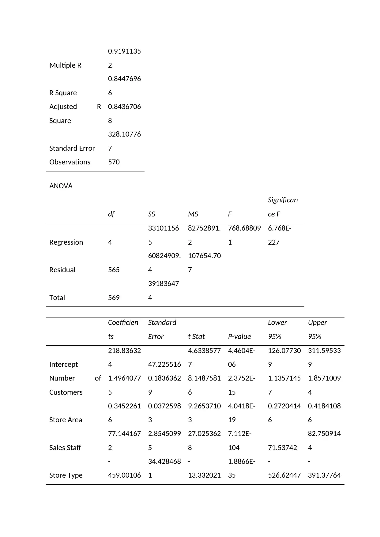
Multiple regression analysis:
SUMMARY OUTPUT
Regression Statistics

Multiple R
0.9191135
2
R Square
0.8447696
6
Adjusted R
Square
0.8436706
8
Standard Error
328.10776
7
Observations 570
ANOVA
df SS MS F
Significan
ce F
Regression 4
33101156
5
82752891.
2
768.68809
1
6.768E-
227
Residual 565
60824909.
4
107654.70
7
Total 569
39183647
4
Coefficien
ts
Standard
Error t Stat P-value
Lower
95%
Upper
95%
Intercept
218.83632
4 47.225516
4.6338577
7
4.4604E-
06
126.07730
9
311.59533
9
Number of
Customers
1.4964077
5
0.1836362
9
8.1487581
6
2.3752E-
15
1.1357145
7
1.8571009
4
Store Area
0.3452261
6
0.0372598
3
9.2653710
3
4.0418E-
19
0.2720414
6
0.4184108
6
Sales Staff
77.144167
2
2.8545099
5
27.025362
8
7.112E-
104 71.53742
82.750914
4
Store Type
-
459.00106
34.428468
1
-
13.332021
1.8866E-
35
-
526.62447
-
391.37764

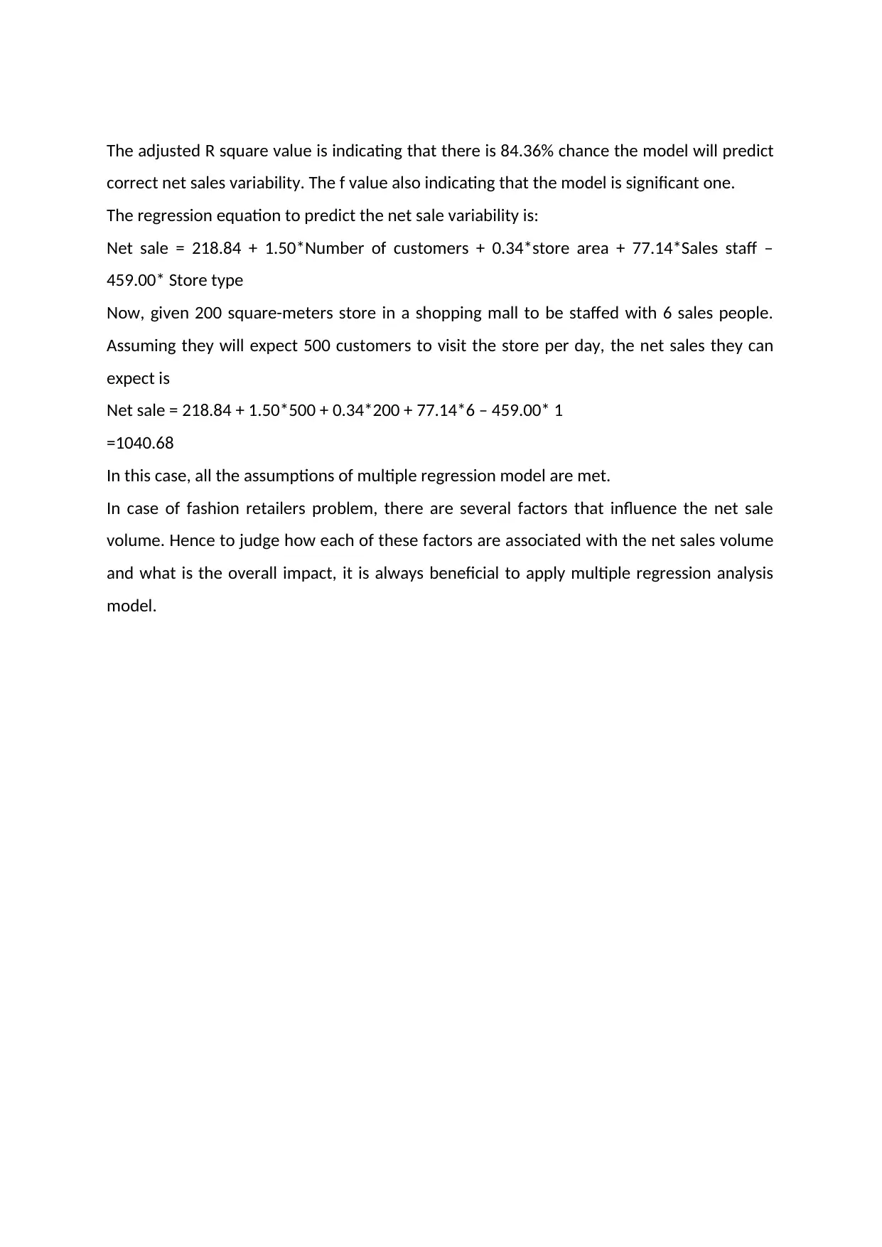
The adjusted R square value is indicating that there is 84.36% chance the model will predict
correct net sales variability. The f value also indicating that the model is significant one.
The regression equation to predict the net sale variability is:
Net sale = 218.84 + 1.50*Number of customers + 0.34*store area + 77.14*Sales staff –
459.00* Store type
Now, given 200 square-meters store in a shopping mall to be staffed with 6 sales people.
Assuming they will expect 500 customers to visit the store per day, the net sales they can
expect is
Net sale = 218.84 + 1.50*500 + 0.34*200 + 77.14*6 – 459.00* 1
=1040.68
In this case, all the assumptions of multiple regression model are met.
In case of fashion retailers problem, there are several factors that influence the net sale
volume. Hence to judge how each of these factors are associated with the net sales volume
and what is the overall impact, it is always beneficial to apply multiple regression analysis
model.