Project 3: Linear-Quadratic Controller and Kalman Filter
VerifiedAdded on 2022/09/09
|9
|605
|18
Project
AI Summary
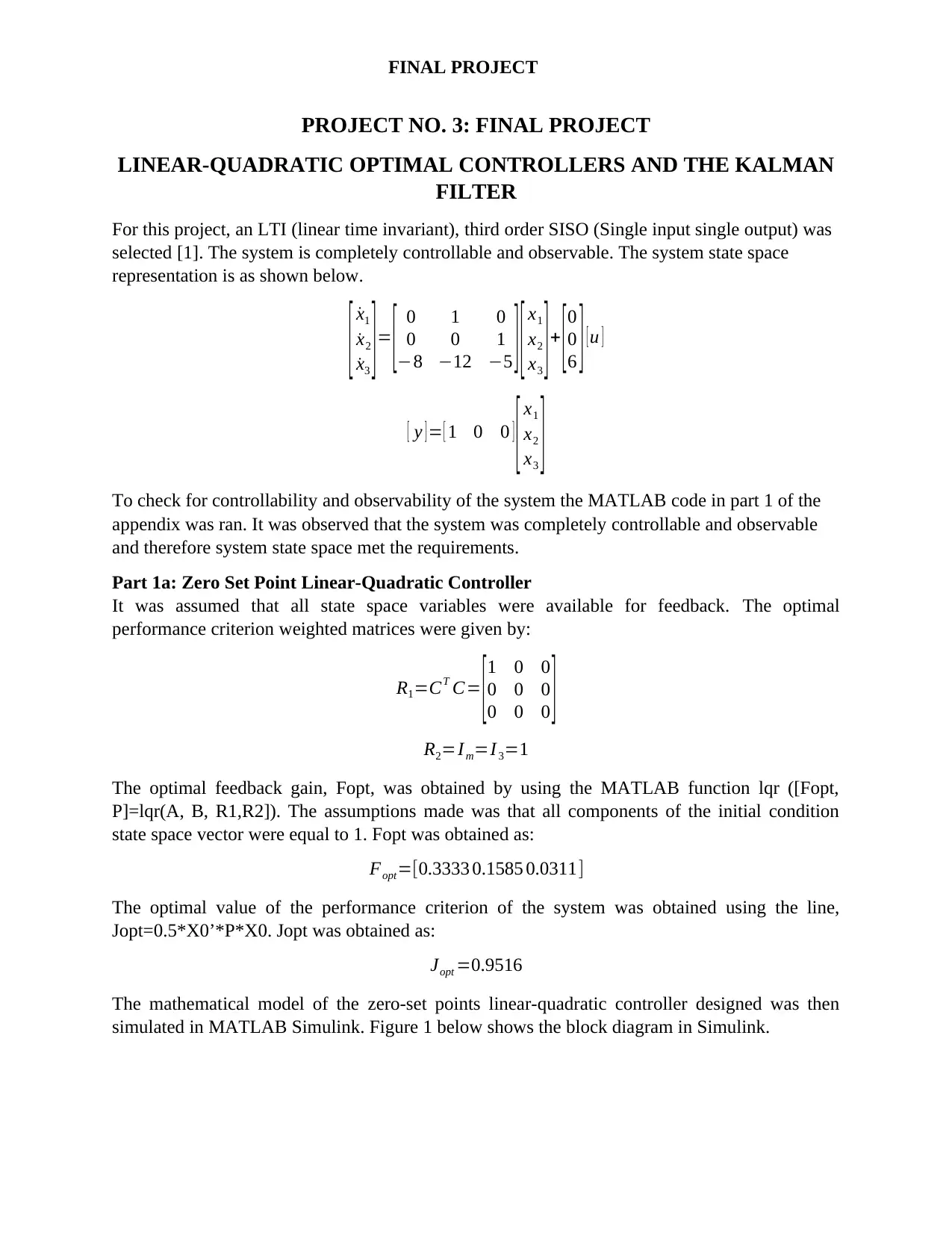
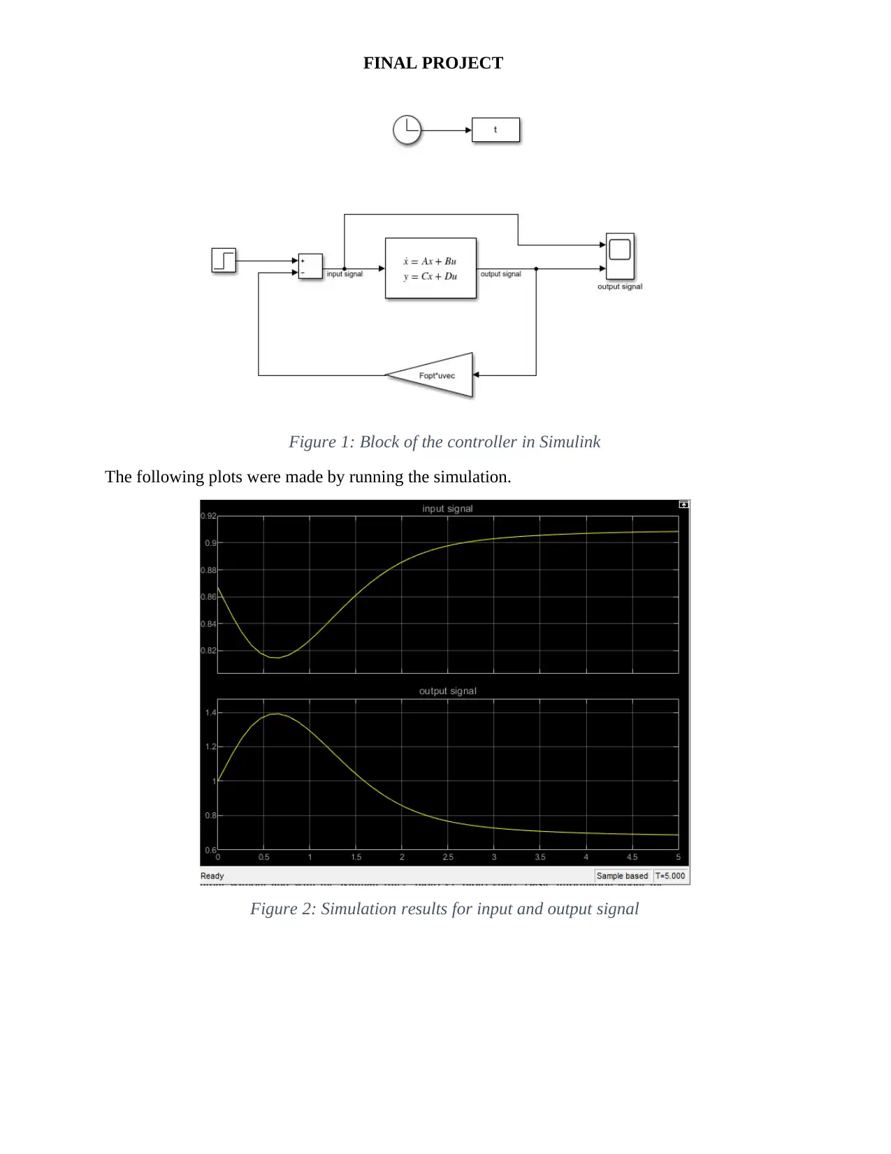
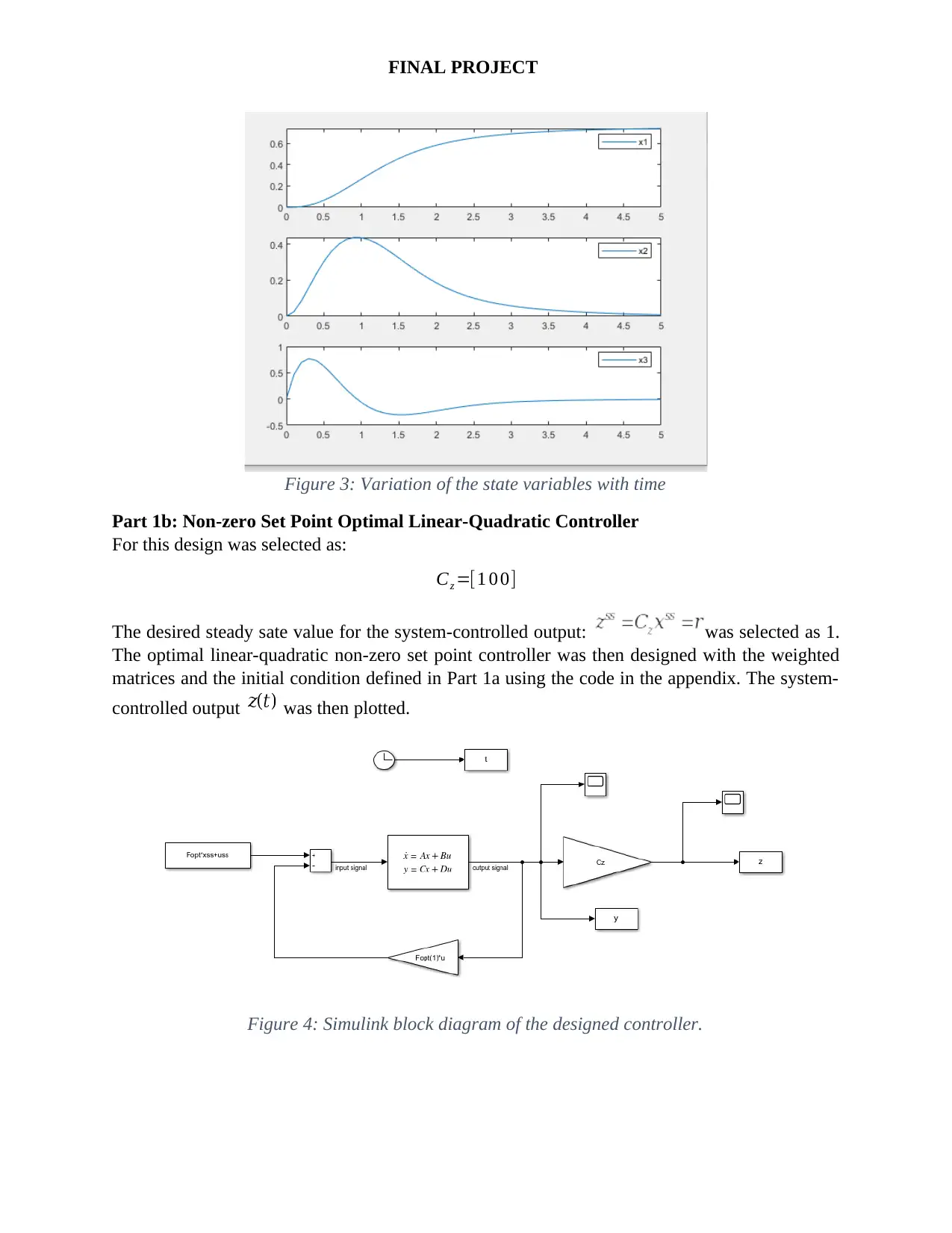
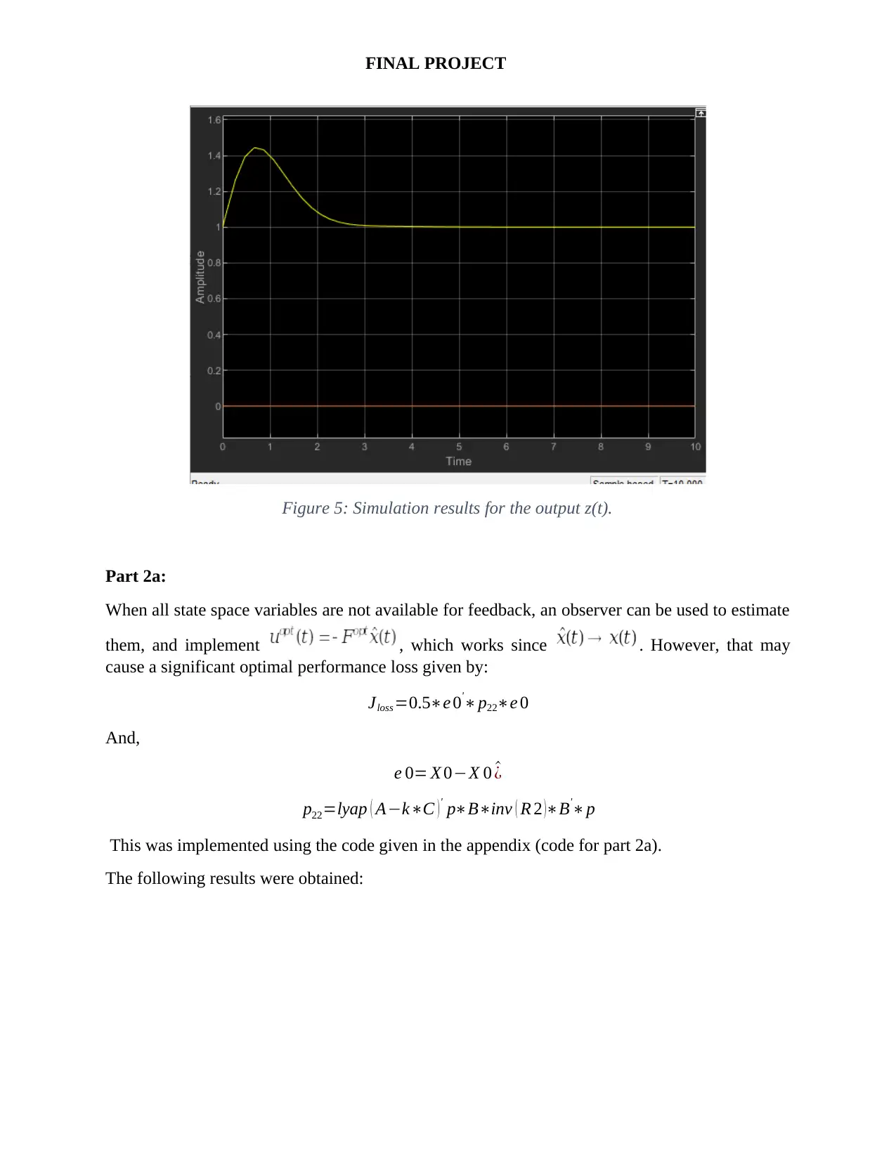
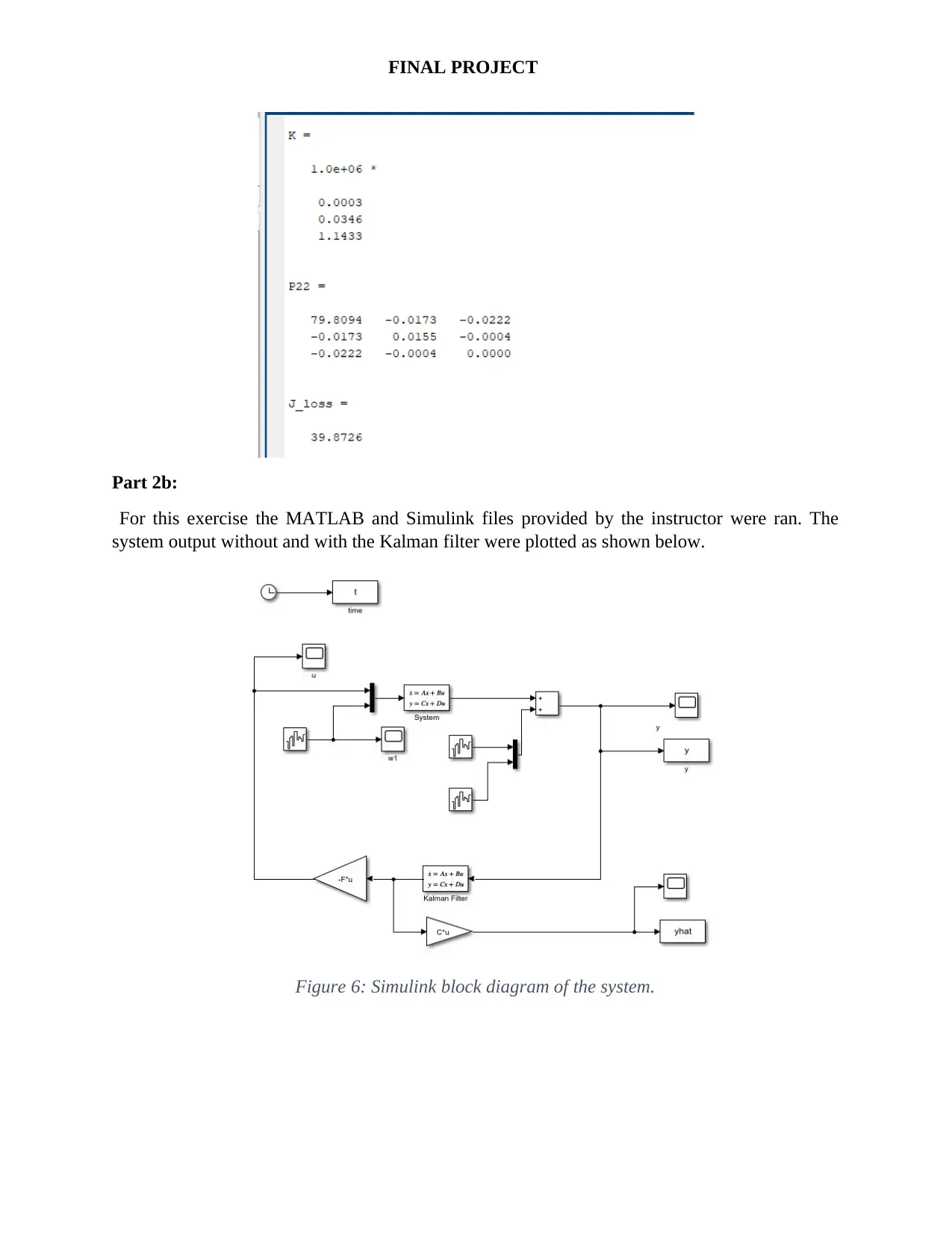
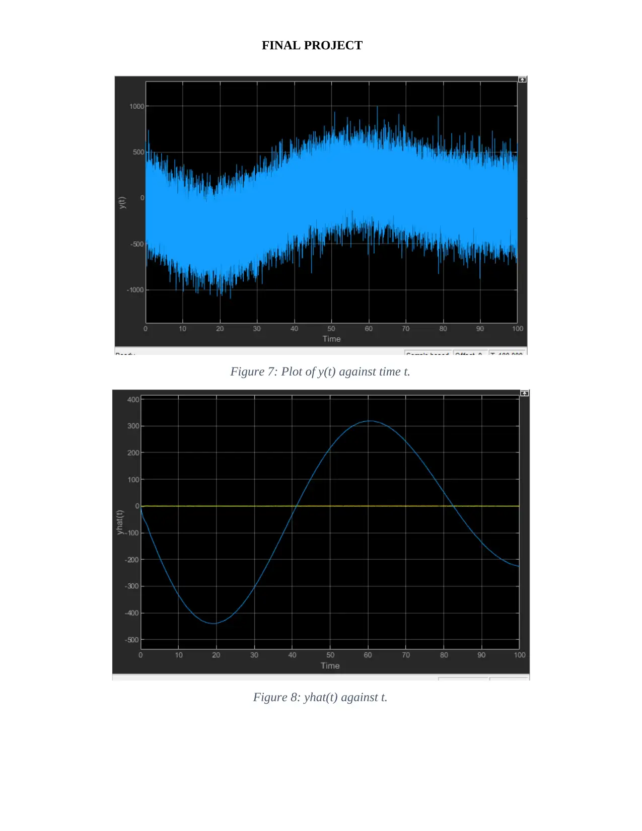
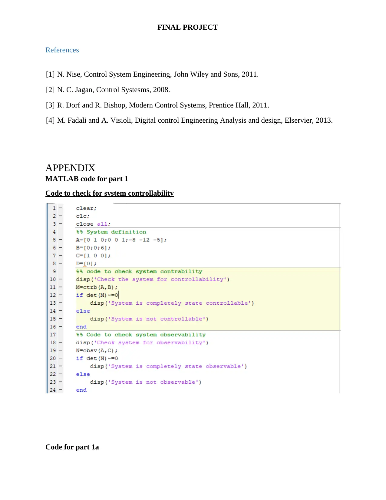
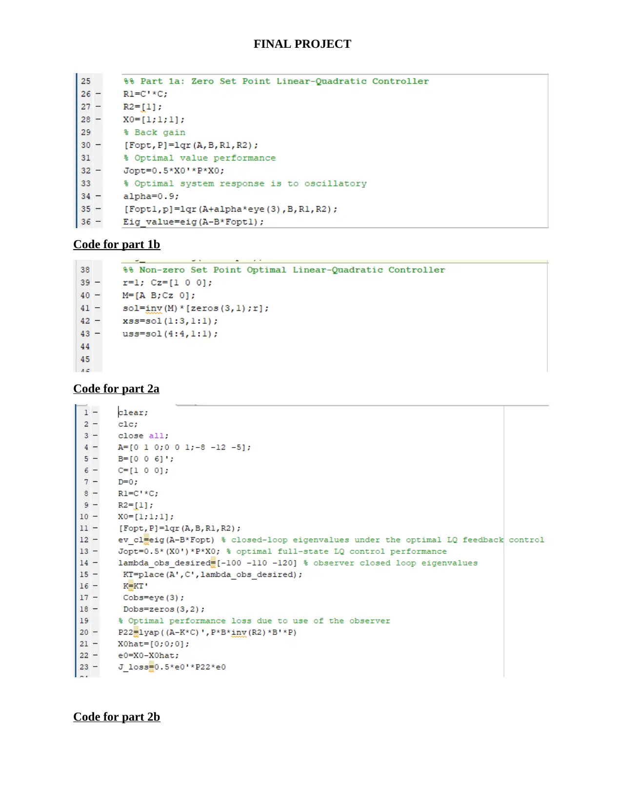
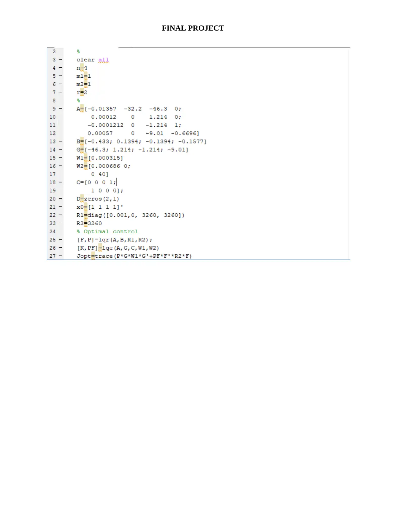
This project focuses on the design and analysis of Linear-Quadratic (LQ) optimal controllers and Kalman filters for a third-order, single-input single-output (SISO) system. The project begins by establishing the system's controllability and observability using MATLAB. Part 1a involves designing a zero-set point LQ controller, determining the optimal feedback gain (Fopt) and the optimal performance criterion (Jopt), and simulating the system in Simulink, with plots of input, output, and state variables. Part 1b extends this to a non-zero set point controller. Part 2a explores the use of an observer when all state space variables are not available for feedback, evaluating the performance loss. Finally, Part 2b utilizes pre-provided MATLAB and Simulink files to analyze system output with and without a Kalman filter, comparing the results. The project incorporates concepts of state-space representation, optimal control theory, and the application of MATLAB and Simulink for simulation and analysis.
1 out of 9
Related Documents


Your All-in-One AI-Powered Toolkit for Academic Success.
+13062052269
info@desklib.com
Available 24*7 on WhatsApp / Email
![[object Object]](/_next/static/media/star-bottom.7253800d.svg)
Copyright © 2020–2026 A2Z Services. All Rights Reserved. Developed and managed by ZUCOL.