Data Analysis Report: Modeling and Predicting Population Growth Trends
VerifiedAdded on 2022/09/09
|11
|1321
|25
Report
AI Summary
This report analyzes population growth data using various mathematical models, including quadratic, cubic, and exponential functions. The analysis begins with creating graphs to visualize the data and assess potential model fits. The study then proceeds to fit the data to the models, evaluating their performance using metrics like R-squared and Sum of Squared Errors (SSE). The models are used to predict future population values, and the accuracy of these predictions is assessed. Furthermore, the report investigates the impact of incorporating additional data points to refine the models and improve their predictive capabilities. The findings indicate that the cubic model initially provides the best fit, but further analysis with expanded data suggests that while the cubic model remains a strong candidate, other models also show promise. The report emphasizes the importance of model selection and the potential for overfitting with limited datasets. References to related research papers are provided to support the analysis and conclusions.

Table of Content
Step One: Creating Graphs.............................................................................................2
Step Two: Fitting the Data.............................................................................................4
Step Three: Making predictions.....................................................................................6
Step Four: Using additional data to update the model...................................................7
References....................................................................................................................11
List of Figures
Figure 1 : Linear Model Plot.............................................................................................2
Figure 2 : 2nd Order Polynomial Plot..............................................................................2
Figure 3 : 3rd Order Polynomial Plot...............................................................................3
Figure 4 : Exponential Model Plot....................................................................................3
Figure 5 : Quadratic Model Fitting...................................................................................4
Figure 6 : Cubic Model Fitting.........................................................................................5
Figure 7 : Exponential Model Fitting................................................................................5
Figure 8 : Quadratic Improved Model Fitting.................................................................8
Figure 9 : Cubic Improved Model Fitting........................................................................8
Figure 10 : Exponential Improved Model Fitting.............................................................9
List of Tables
Table 1 : Initial Models and their Performance................................................................6
Table 2 : Improved Models and their Performance..........................................................9
Paraphrase This Document
Need a fresh take? Get an instant paraphrase of this document with our AI Paraphraser
1
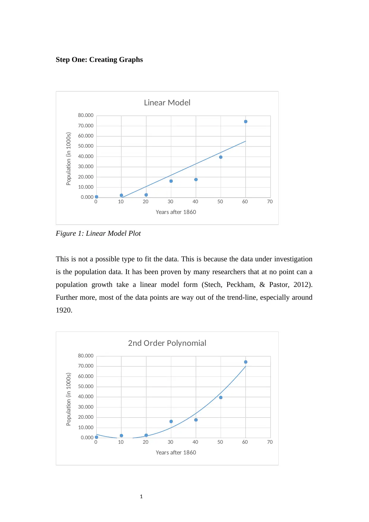
Step One: Creating Graphs
0 10 20 30 40 50 60 70
0.000
10.000
20.000
30.000
40.000
50.000
60.000
70.000
80.000
Linear Model
Years after 1860
Population (in 1000s)
Figure 1: Linear Model Plot
This is not a possible type to fit the data. This is because the data under investigation
is the population data. It has been proven by many researchers that at no point can a
population growth take a linear model form (Stech, Peckham, & Pastor, 2012).
Further more, most of the data points are way out of the trend-line, especially around
1920.
0 10 20 30 40 50 60 70
0.000
10.000
20.000
30.000
40.000
50.000
60.000
70.000
80.000
2nd Order Polynomial
Years after 1860
Population (in 1000s)
2
Figure 2: 2nd Order Polynomial Plot
This could be a possible fit base on the trend-line. However, the tendency of the
population returning back to zero around the 10th year is abnormal and discredits this
curve as a possible fit (Patel, Khurana, Sharma, Kumar, & Ragumani, 2018).
0 10 20 30 40 50 60 70
0.000
10.000
20.000
30.000
40.000
50.000
60.000
70.000
80.000
3rd Order Polynomial
Years after 1860
Population (in 1000s)
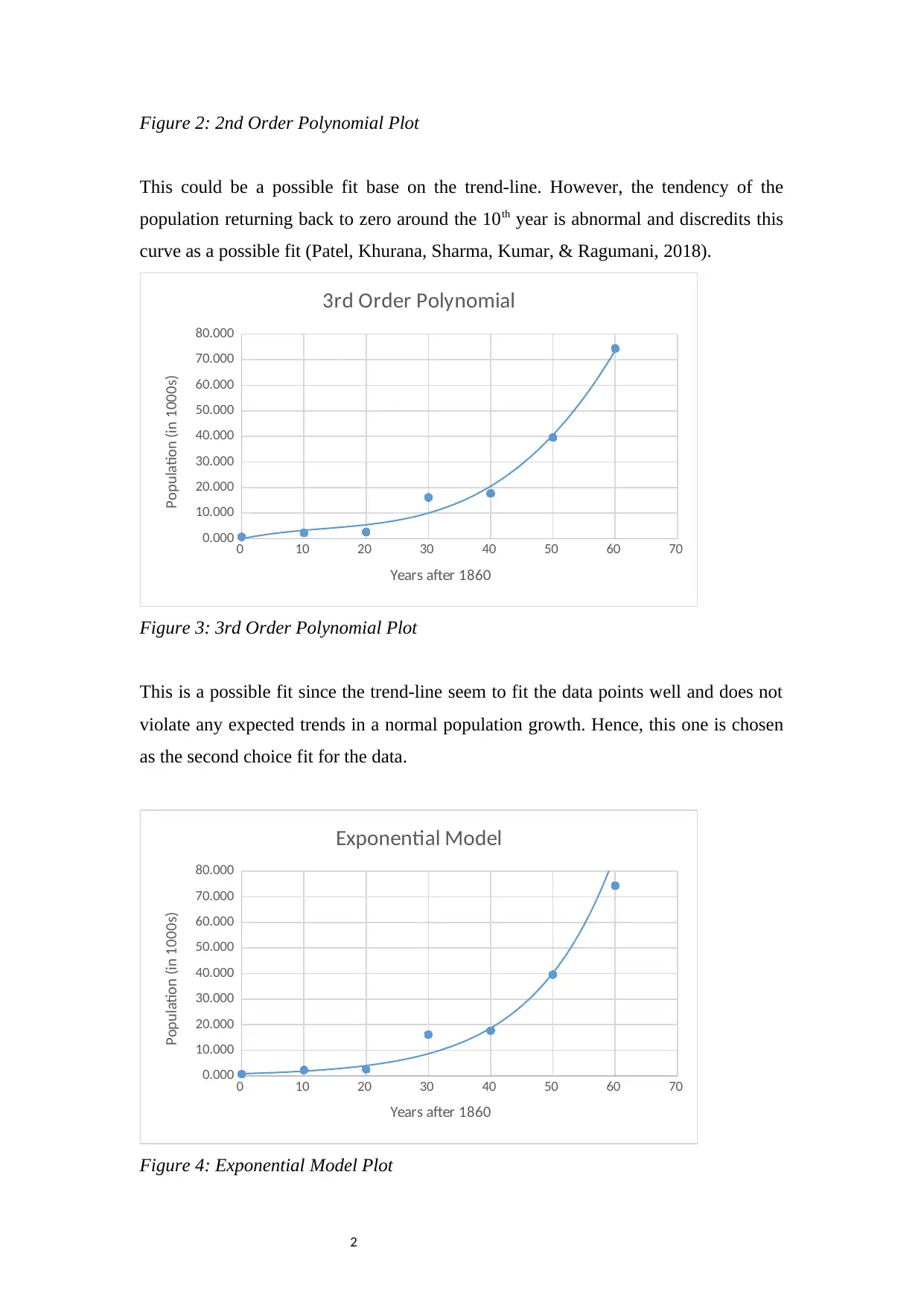
Figure 3: 3rd Order Polynomial Plot
This is a possible fit since the trend-line seem to fit the data points well and does not
violate any expected trends in a normal population growth. Hence, this one is chosen
as the second choice fit for the data.
0 10 20 30 40 50 60 70
0.000
10.000
20.000
30.000
40.000
50.000
60.000
70.000
80.000
Exponential Model
Years after 1860
Population (in 1000s)
Figure 4: Exponential Model Plot
Figure 2: 2nd Order Polynomial Plot
This could be a possible fit base on the trend-line. However, the tendency of the
population returning back to zero around the 10th year is abnormal and discredits this
curve as a possible fit (Patel, Khurana, Sharma, Kumar, & Ragumani, 2018).
0 10 20 30 40 50 60 70
0.000
10.000
20.000
30.000
40.000
50.000
60.000
70.000
80.000
3rd Order Polynomial
Years after 1860
Population (in 1000s)
Figure 3: 3rd Order Polynomial Plot
This is a possible fit since the trend-line seem to fit the data points well and does not
violate any expected trends in a normal population growth. Hence, this one is chosen
as the second choice fit for the data.
0 10 20 30 40 50 60 70
0.000
10.000
20.000
30.000
40.000
50.000
60.000
70.000
80.000
Exponential Model
Years after 1860
Population (in 1000s)
Figure 4: Exponential Model Plot
⊘ This is a preview!⊘
Do you want full access?
Subscribe today to unlock all pages.
Trusted by 1+ million students worldwide
3
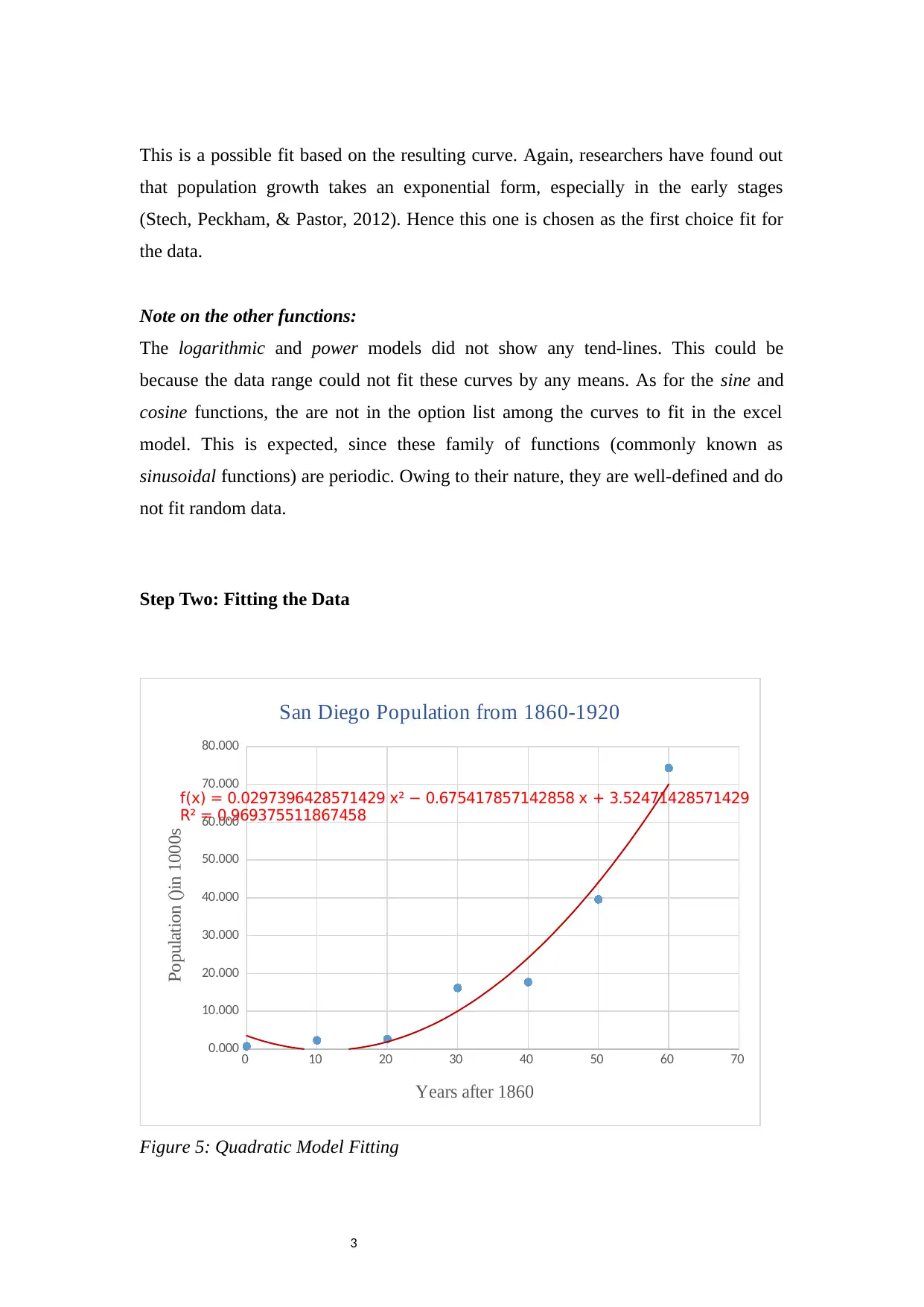
This is a possible fit based on the resulting curve. Again, researchers have found out
that population growth takes an exponential form, especially in the early stages
(Stech, Peckham, & Pastor, 2012). Hence this one is chosen as the first choice fit for
the data.
Note on the other functions:
The logarithmic and power models did not show any tend-lines. This could be
because the data range could not fit these curves by any means. As for the sine and
cosine functions, the are not in the option list among the curves to fit in the excel
model. This is expected, since these family of functions (commonly known as
sinusoidal functions) are periodic. Owing to their nature, they are well-defined and do
not fit random data.
Step Two: Fitting the Data
0 10 20 30 40 50 60 70
0.000
10.000
20.000
30.000
40.000
50.000
60.000
70.000
80.000
f(x) = 0.0297396428571429 x² − 0.675417857142858 x + 3.52471428571429
R² = 0.969375511867458
San Diego Population from 1860-1920
Years after 1860
Population ()in 1000s
Figure 5: Quadratic Model Fitting
Paraphrase This Document
Need a fresh take? Get an instant paraphrase of this document with our AI Paraphraser
4
0 10 20 30 40 50 60 70
0.000
10.000
20.000
30.000
40.000
50.000
60.000
70.000
80.000
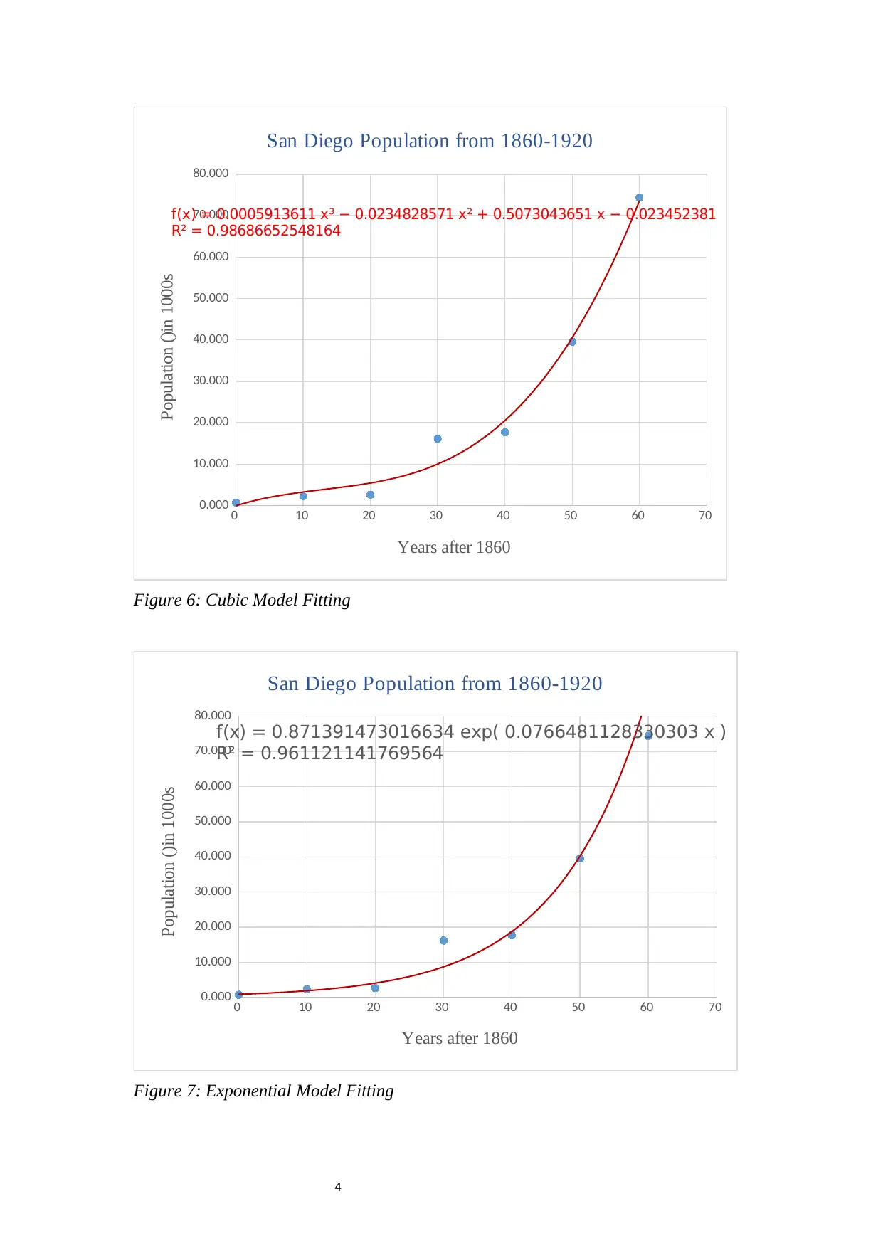
f(x) = 0.0005913611 x³ − 0.0234828571 x² + 0.5073043651 x − 0.023452381
R² = 0.98686652548164
San Diego Population from 1860-1920
Years after 1860
Population ()in 1000s
Figure 6: Cubic Model Fitting
0 10 20 30 40 50 60 70
0.000
10.000
20.000
30.000
40.000
50.000
60.000
70.000
80.000
f(x) = 0.871391473016634 exp( 0.0766481128330303 x )
R² = 0.961121141769564
San Diego Population from 1860-1920
Years after 1860
Population ()in 1000s
Figure 7: Exponential Model Fitting
0 10 20 30 40 50 60 70
0.000
10.000
20.000
30.000
40.000
50.000
60.000
70.000
80.000
f(x) = 0.0005913611 x³ − 0.0234828571 x² + 0.5073043651 x − 0.023452381
R² = 0.98686652548164
San Diego Population from 1860-1920
Years after 1860
Population ()in 1000s
Figure 6: Cubic Model Fitting
0 10 20 30 40 50 60 70
0.000
10.000
20.000
30.000
40.000
50.000
60.000
70.000
80.000
f(x) = 0.871391473016634 exp( 0.0766481128330303 x )
R² = 0.961121141769564
San Diego Population from 1860-1920
Years after 1860
Population ()in 1000s
Figure 7: Exponential Model Fitting
5
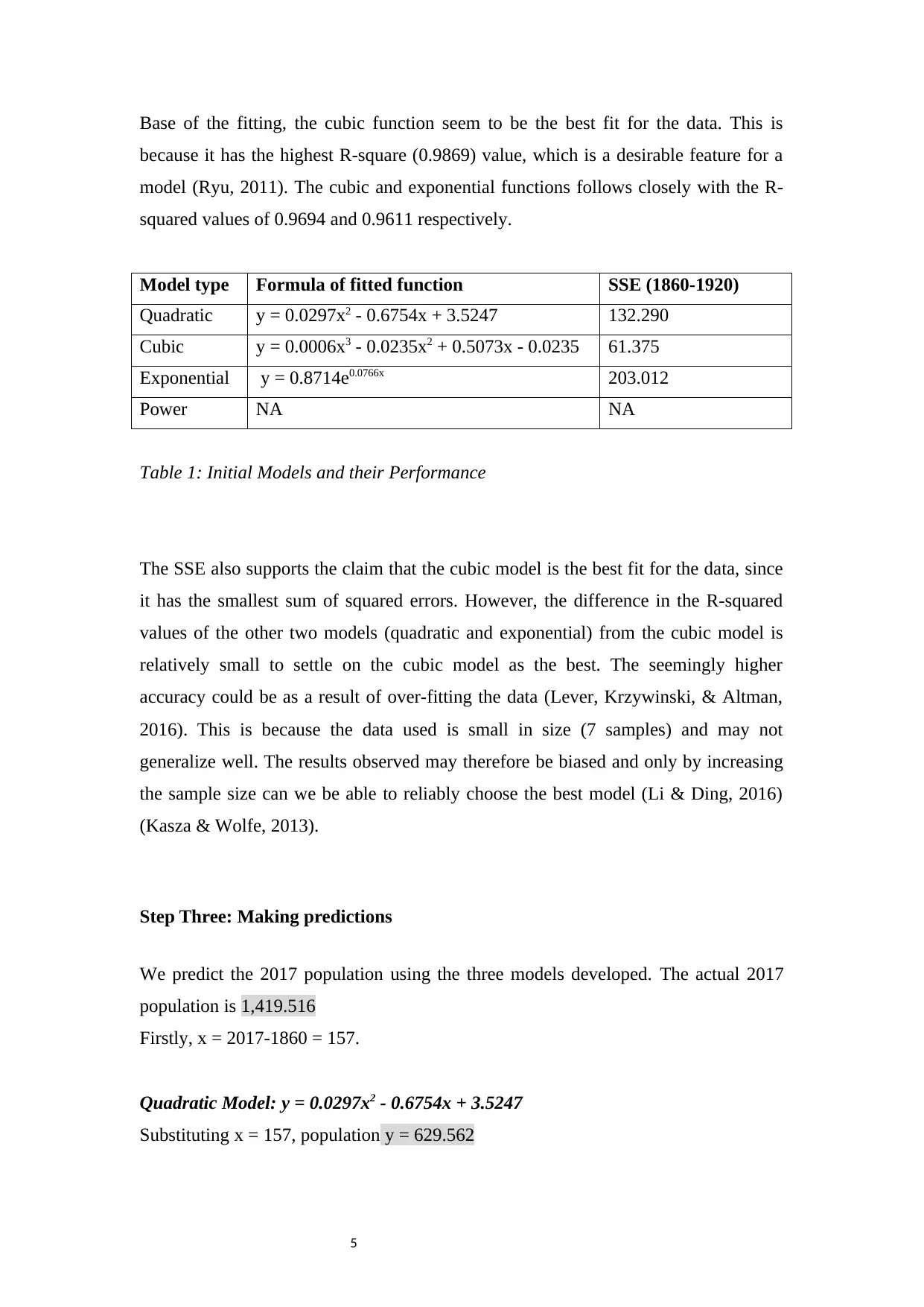
Base of the fitting, the cubic function seem to be the best fit for the data. This is
because it has the highest R-square (0.9869) value, which is a desirable feature for a
model (Ryu, 2011). The cubic and exponential functions follows closely with the R-
squared values of 0.9694 and 0.9611 respectively.
Model type Formula of fitted function SSE (1860-1920)
Quadratic y = 0.0297x2 - 0.6754x + 3.5247 132.290
Cubic y = 0.0006x3 - 0.0235x2 + 0.5073x - 0.0235 61.375
Exponential y = 0.8714e0.0766x 203.012
Power NA NA
Table 1: Initial Models and their Performance
The SSE also supports the claim that the cubic model is the best fit for the data, since
it has the smallest sum of squared errors. However, the difference in the R-squared
values of the other two models (quadratic and exponential) from the cubic model is
relatively small to settle on the cubic model as the best. The seemingly higher
accuracy could be as a result of over-fitting the data (Lever, Krzywinski, & Altman,
2016). This is because the data used is small in size (7 samples) and may not
generalize well. The results observed may therefore be biased and only by increasing
the sample size can we be able to reliably choose the best model (Li & Ding, 2016)
(Kasza & Wolfe, 2013).
Step Three: Making predictions
We predict the 2017 population using the three models developed. The actual 2017
population is 1,419.516
Firstly, x = 2017-1860 = 157.
Quadratic Model: y = 0.0297x2 - 0.6754x + 3.5247
Substituting x = 157, population y = 629.562
⊘ This is a preview!⊘
Do you want full access?
Subscribe today to unlock all pages.
Trusted by 1+ million students worldwide
6
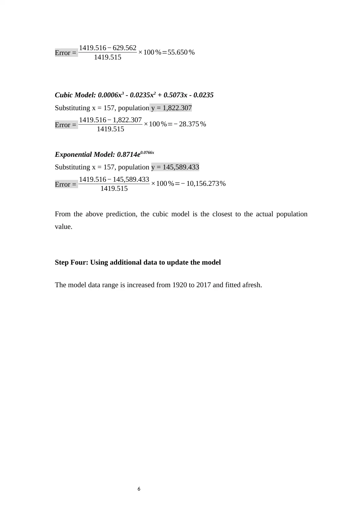
Error = 1419.516− 629.562
1419.515 ×100 %=55.650 %
Cubic Model: 0.0006x3 - 0.0235x2 + 0.5073x - 0.0235
Substituting x = 157, population y = 1,822.307
Error = 1419.516− 1,822.307
1419.515 ×100 %=− 28.375 %
Exponential Model: 0.8714e0.0766x
Substituting x = 157, population y = 145,589.433
Error = 1419.516− 145,589.433
1419.515 ×100 %=− 10,156.273%
From the above prediction, the cubic model is the closest to the actual population
value.
Step Four: Using additional data to update the model
The model data range is increased from 1920 to 2017 and fitted afresh.
Paraphrase This Document
Need a fresh take? Get an instant paraphrase of this document with our AI Paraphraser
7
0 20 40 60 80 100 120 140 160 180
0.000
200.000
400.000
600.000
800.000
1,000.000
1,200.000
1,400.000
1,600.000
f(x) = 0.0724591997105615 x² − 1.98091100302872 x − 11.4898269196452
R² = 0.990826133015843
San Diego Population from 1860-2017
Years after 1860
Population (in 100s)
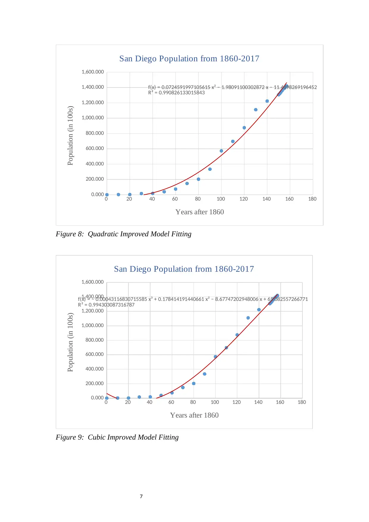
Figure 8: Quadratic Improved Model Fitting
0 20 40 60 80 100 120 140 160 180
0.000
200.000
400.000
600.000
800.000
1,000.000
1,200.000
1,400.000
1,600.000
f(x) = − 0.00043116830715585 x³ + 0.178414191440661 x² − 8.67747202948006 x + 65.082557266771
R² = 0.994303087316787
San Diego Population from 1860-2017
Years after 1860
Population (in 100s)
Figure 9: Cubic Improved Model Fitting
0 20 40 60 80 100 120 140 160 180
0.000
200.000
400.000
600.000
800.000
1,000.000
1,200.000
1,400.000
1,600.000
f(x) = 0.0724591997105615 x² − 1.98091100302872 x − 11.4898269196452
R² = 0.990826133015843
San Diego Population from 1860-2017
Years after 1860
Population (in 100s)
Figure 8: Quadratic Improved Model Fitting
0 20 40 60 80 100 120 140 160 180
0.000
200.000
400.000
600.000
800.000
1,000.000
1,200.000
1,400.000
1,600.000
f(x) = − 0.00043116830715585 x³ + 0.178414191440661 x² − 8.67747202948006 x + 65.082557266771
R² = 0.994303087316787
San Diego Population from 1860-2017
Years after 1860
Population (in 100s)
Figure 9: Cubic Improved Model Fitting
8
0 20 40 60 80 100 120 140 160 180
0.000
200.000
400.000
600.000
800.000
1,000.000
1,200.000
1,400.000
1,600.000 f(x) = 3.06454006800282 exp( 0.0425998658064206 x )
R² = 0.921462407973523
San Diego Population from 1860-2017
Years after 1860
Population (in 100s)
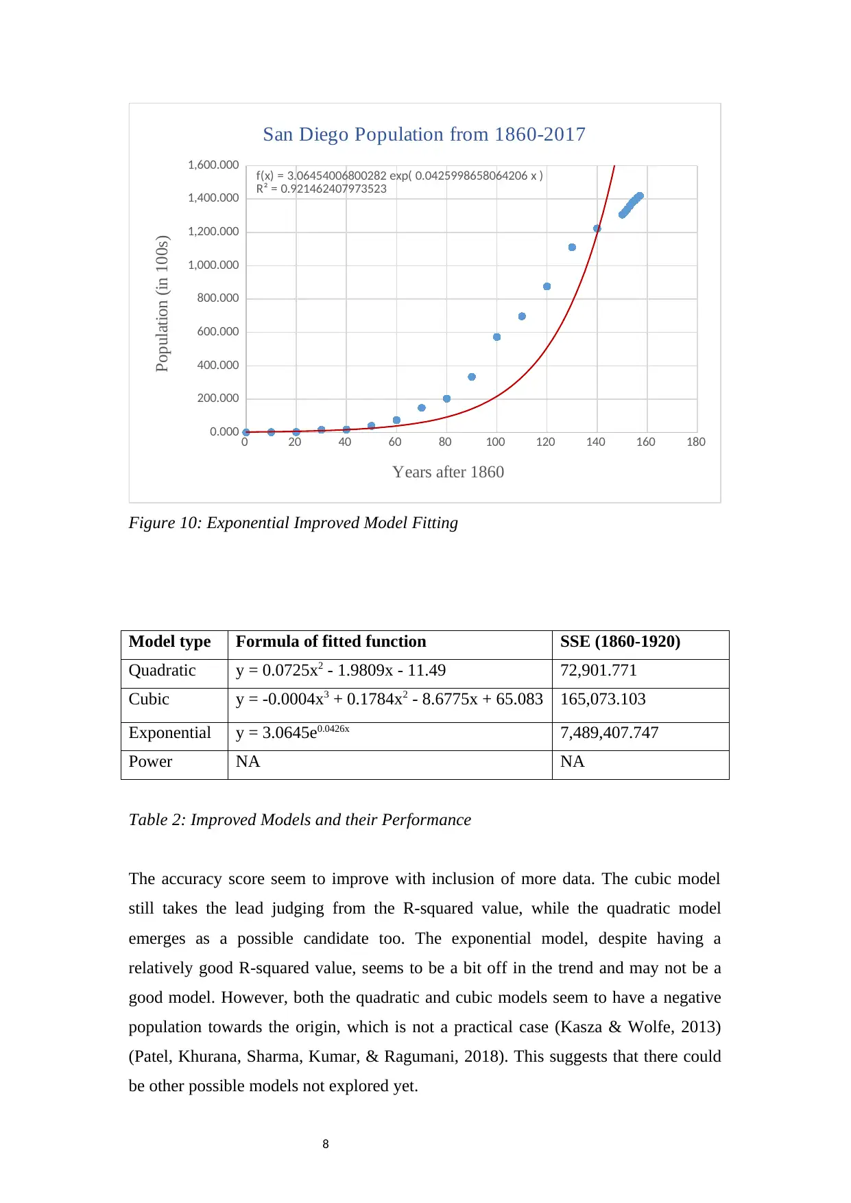
Figure 10: Exponential Improved Model Fitting
Model type Formula of fitted function SSE (1860-1920)
Quadratic y = 0.0725x2 - 1.9809x - 11.49 72,901.771
Cubic y = -0.0004x3 + 0.1784x2 - 8.6775x + 65.083 165,073.103
Exponential y = 3.0645e0.0426x 7,489,407.747
Power NA NA
Table 2: Improved Models and their Performance
The accuracy score seem to improve with inclusion of more data. The cubic model
still takes the lead judging from the R-squared value, while the quadratic model
emerges as a possible candidate too. The exponential model, despite having a
relatively good R-squared value, seems to be a bit off in the trend and may not be a
good model. However, both the quadratic and cubic models seem to have a negative
population towards the origin, which is not a practical case (Kasza & Wolfe, 2013)
(Patel, Khurana, Sharma, Kumar, & Ragumani, 2018). This suggests that there could
be other possible models not explored yet.
0 20 40 60 80 100 120 140 160 180
0.000
200.000
400.000
600.000
800.000
1,000.000
1,200.000
1,400.000
1,600.000 f(x) = 3.06454006800282 exp( 0.0425998658064206 x )
R² = 0.921462407973523
San Diego Population from 1860-2017
Years after 1860
Population (in 100s)
Figure 10: Exponential Improved Model Fitting
Model type Formula of fitted function SSE (1860-1920)
Quadratic y = 0.0725x2 - 1.9809x - 11.49 72,901.771
Cubic y = -0.0004x3 + 0.1784x2 - 8.6775x + 65.083 165,073.103
Exponential y = 3.0645e0.0426x 7,489,407.747
Power NA NA
Table 2: Improved Models and their Performance
The accuracy score seem to improve with inclusion of more data. The cubic model
still takes the lead judging from the R-squared value, while the quadratic model
emerges as a possible candidate too. The exponential model, despite having a
relatively good R-squared value, seems to be a bit off in the trend and may not be a
good model. However, both the quadratic and cubic models seem to have a negative
population towards the origin, which is not a practical case (Kasza & Wolfe, 2013)
(Patel, Khurana, Sharma, Kumar, & Ragumani, 2018). This suggests that there could
be other possible models not explored yet.
⊘ This is a preview!⊘
Do you want full access?
Subscribe today to unlock all pages.
Trusted by 1+ million students worldwide

9
Paraphrase This Document
Need a fresh take? Get an instant paraphrase of this document with our AI Paraphraser
10
References
Kasza, J., & Wolfe, R. (2013). Interpretation of commonly used statistical regression
models. Respirology, 19(1), 14–21. https://doi.org/10.1111/resp.12221
Lever, J., Krzywinski, M., & Altman, N. (2016). Model selection and overfitting.
Nature Methods, 13(9), 703–704. https://doi.org/10.1038/nmeth.3968
Li, Y., & Ding, C. (2016). Effects of Sample Size, Sample Accuracy and
Environmental Variables on Predictive Performance of MaxEnt Model. Polish
Journal of Ecology, 64(3), 303–312.
https://doi.org/10.3161/15052249pje2016.64.3.001
Patel, J. C., Khurana, P., Sharma, Y. K., Kumar, B., & Ragumani, S. (2018). Chronic
lifestyle diseases display seasonal sensitive comorbid trend in human
population evidence from Google Trends. PLOS ONE, 13(12), e0207359.
https://doi.org/10.1371/journal.pone.0207359
Ryu, H. K. (2011). Subjective model selection rules versus passive model selection
rules. Economic Modelling, 28(1–2), 459–472.
https://doi.org/10.1016/j.econmod.2010.08.002
Stech, H., Peckham, B., & Pastor, J. (2012). Enrichment in a general class of
stoichiometric producer–consumer population growth models. Theoretical
Population Biology, 81(3), 210–222. https://doi.org/10.1016/j.tpb.2012.01.003
1 out of 11

Your All-in-One AI-Powered Toolkit for Academic Success.
+13062052269
info@desklib.com
Available 24*7 on WhatsApp / Email
![[object Object]](/_next/static/media/star-bottom.7253800d.svg)
Unlock your academic potential
Copyright © 2020–2026 A2Z Services. All Rights Reserved. Developed and managed by ZUCOL.