MA209 Homework 2: Numerical Methods, Interpolation Techniques
VerifiedAdded on 2022/08/19
|11
|1197
|14
Homework Assignment
AI Summary
This document presents a complete solution to MA209 Homework 2, focusing on numerical methods for solving ordinary differential equations (ODEs) and polynomial interpolation. The solution includes detailed explanations and MATLAB code implementations for various numerical techniques, such as the modified Euler's method (Heun's algorithm) to solve an initial value problem. The document also analyzes the error tolerance and step size in the context of the algorithm. Furthermore, it explores a population model using Euler's method and discusses the limiting values of the system. Finally, the solution demonstrates polynomial interpolation using the direct method to fit a given dataset and calculates the roots of the resulting polynomial function. The solution is a comprehensive resource for understanding and applying numerical methods and interpolation techniques.
Running head: MA209 HOMEWORK 2
MA209 HOMEWORK 2
Name of the Student
Name of the University
Author Note
MA209 HOMEWORK 2
Name of the Student
Name of the University
Author Note
Paraphrase This Document
Need a fresh take? Get an instant paraphrase of this document with our AI Paraphraser
1MA209 HOMEWORK 2
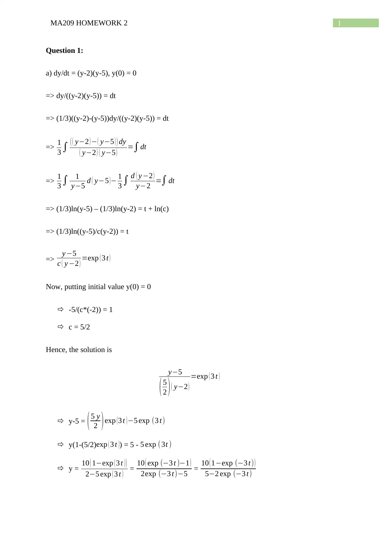
Question 1:
a) dy/dt = (y-2)(y-5), y(0) = 0
=> dy/((y-2)(y-5)) = dt
=> (1/3)((y-2)-(y-5))dy/((y-2)(y-5)) = dt
=> 1
3 ∫ ( ( y−2 ) − ( y−5 ) ) dy
( y−2 ) ( y−5 ) =∫dt
=> 1
3 ∫ 1
y−5 d ( y−5 )− 1
3 ∫ d ( y −2 )
y−2 =∫ dt
=> (1/3)ln(y-5) – (1/3)ln(y-2) = t + ln(c)
=> (1/3)ln((y-5)/c(y-2)) = t
=> y −5
c ( y −2 ) =exp ( 3 t )
Now, putting initial value y(0) = 0
-5/(c*(-2)) = 1
c = 5/2
Hence, the solution is
y−5
( 5
2 ) ( y−2 )
=exp ( 3 t )
y-5 = ( 5 y
2 )exp (3 t )−5 exp (3 t)
y(1-(5/2)exp ( 3 t )) = 5 - 5 exp (3t )
y = 10 ( 1−exp ( 3 t ) )
2−5 exp ( 3 t ) = 10 ( exp (−3 t )−1 )
2exp (−3 t)−5 = 10 ( 1−exp (−3 t ) )
5−2 exp (−3 t)
2MA209 HOMEWORK 2
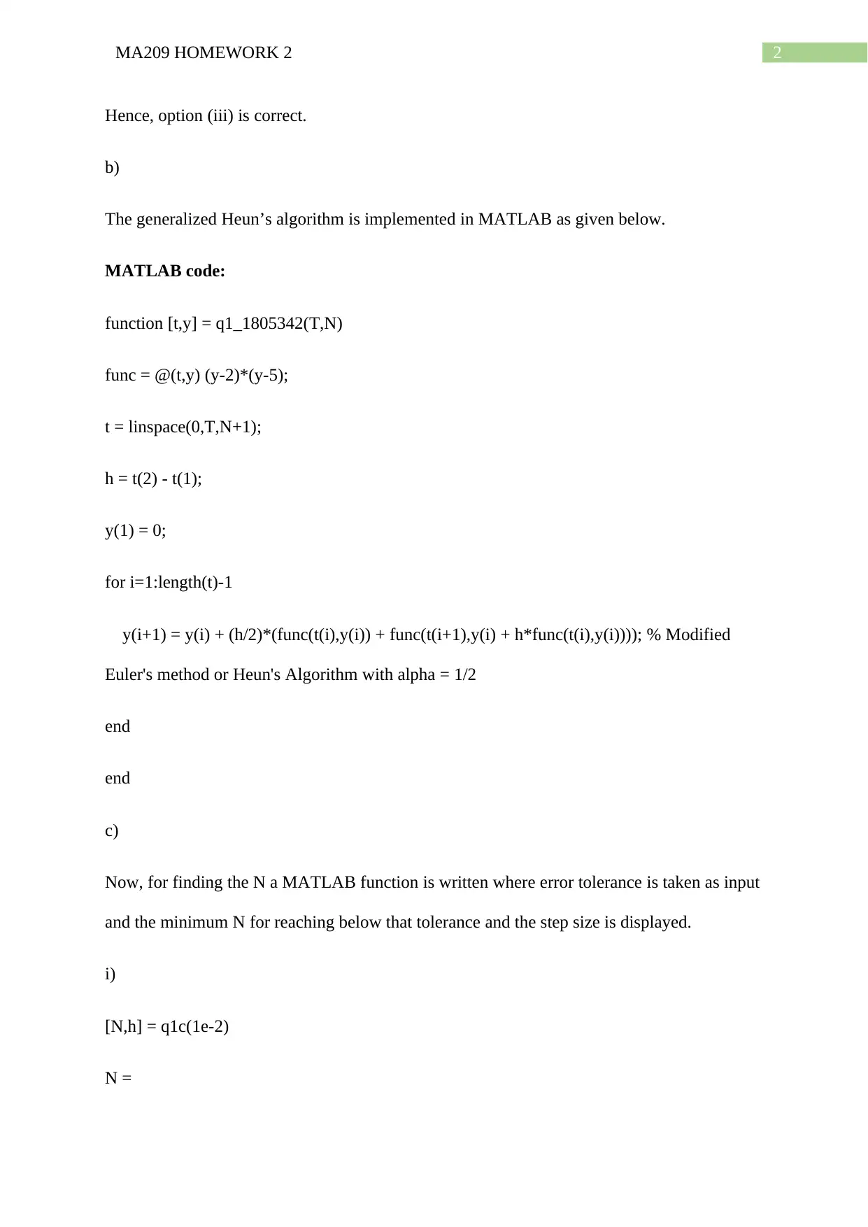
Hence, option (iii) is correct.
b)
The generalized Heun’s algorithm is implemented in MATLAB as given below.
MATLAB code:
function [t,y] = q1_1805342(T,N)
func = @(t,y) (y-2)*(y-5);
t = linspace(0,T,N+1);
h = t(2) - t(1);
y(1) = 0;
for i=1:length(t)-1
y(i+1) = y(i) + (h/2)*(func(t(i),y(i)) + func(t(i+1),y(i) + h*func(t(i),y(i)))); % Modified
Euler's method or Heun's Algorithm with alpha = 1/2
end
end
c)
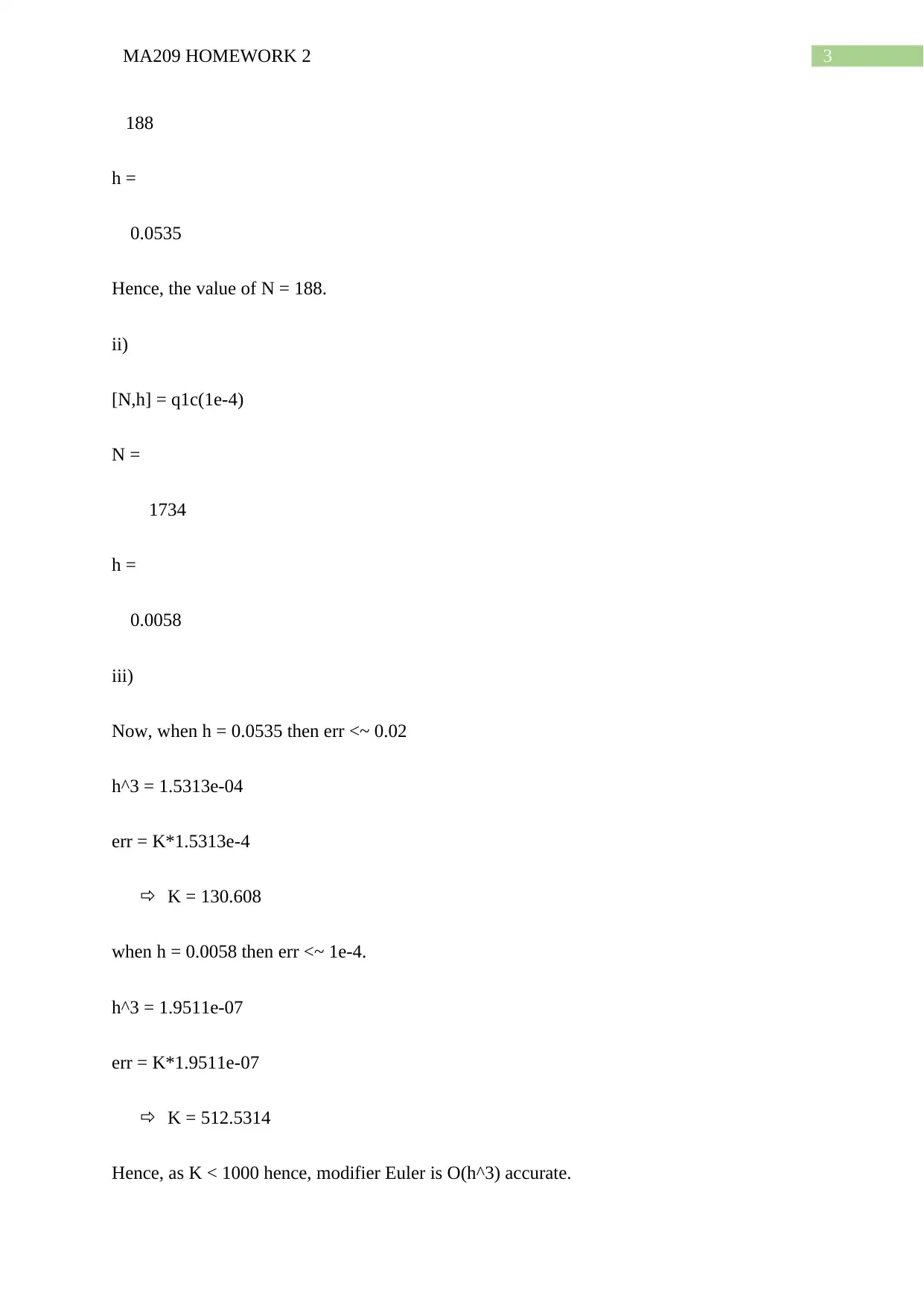
Now, for finding the N a MATLAB function is written where error tolerance is taken as input
and the minimum N for reaching below that tolerance and the step size is displayed.
i)
[N,h] = q1c(1e-2)
N =
⊘ This is a preview!⊘
Do you want full access?
Subscribe today to unlock all pages.

Trusted by 1+ million students worldwide
3MA209 HOMEWORK 2
188
h =
0.0535
Hence, the value of N = 188.
ii)
[N,h] = q1c(1e-4)
N =
1734
h =
0.0058
iii)
Now, when h = 0.0535 then err <~ 0.02
h^3 = 1.5313e-04
err = K*1.5313e-4
K = 130.608
when h = 0.0058 then err <~ 1e-4.
h^3 = 1.9511e-07
err = K*1.9511e-07
K = 512.5314
Hence, as K < 1000 hence, modifier Euler is O(h^3) accurate.
Paraphrase This Document
Need a fresh take? Get an instant paraphrase of this document with our AI Paraphraser
4MA209 HOMEWORK 2
Hence,
Err <~ O(h^3)
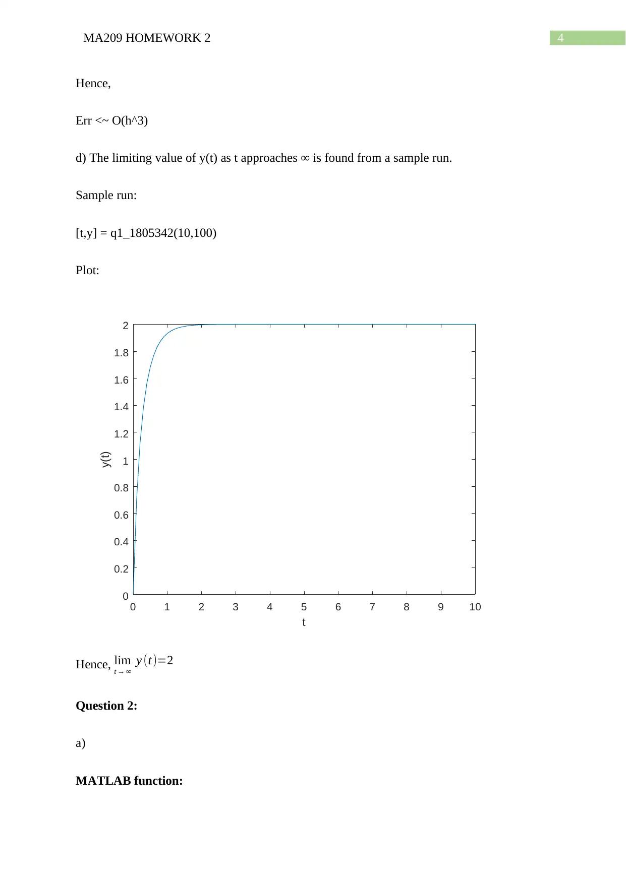
d) The limiting value of y(t) as t approaches ∞ is found from a sample run.
Sample run:
[t,y] = q1_1805342(10,100)
Plot:
0 1 2 3 4 5 6 7 8 9 10
t
0
0.2
0.4
0.6
0.8
1
1.2
1.4
1.6
1.8
2
y(t)
Hence, lim
t → ∞
y (t)=2
Question 2:
a)
MATLAB function:
Hence,
Err <~ O(h^3)
d) The limiting value of y(t) as t approaches ∞ is found from a sample run.
Sample run:
[t,y] = q1_1805342(10,100)
Plot:
0 1 2 3 4 5 6 7 8 9 10
t
0
0.2
0.4
0.6
0.8
1
1.2
1.4
1.6
1.8
2
y(t)
Hence, lim
t → ∞
y (t)=2
Question 2:
a)
MATLAB function:
5MA209 HOMEWORK 2
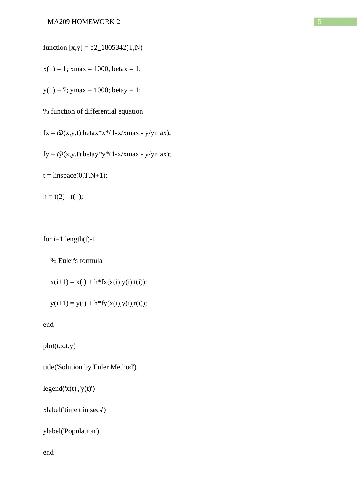
function [x,y] = q2_1805342(T,N)
x(1) = 1; xmax = 1000; betax = 1;
y(1) = 7; ymax = 1000; betay = 1;
% function of differential equation
fx = @(x,y,t) betax*x*(1-x/xmax - y/ymax);
fy = @(x,y,t) betay*y*(1-x/xmax - y/ymax);
t = linspace(0,T,N+1);
h = t(2) - t(1);
for i=1:length(t)-1
% Euler's formula
x(i+1) = x(i) + h*fx(x(i),y(i),t(i));
y(i+1) = y(i) + h*fy(x(i),y(i),t(i));
end
plot(t,x,t,y)
title('Solution by Euler Method')
legend('x(t)','y(t)')
xlabel('time t in secs')
ylabel('Population')
end
⊘ This is a preview!⊘
Do you want full access?
Subscribe today to unlock all pages.

Trusted by 1+ million students worldwide
6MA209 HOMEWORK 2
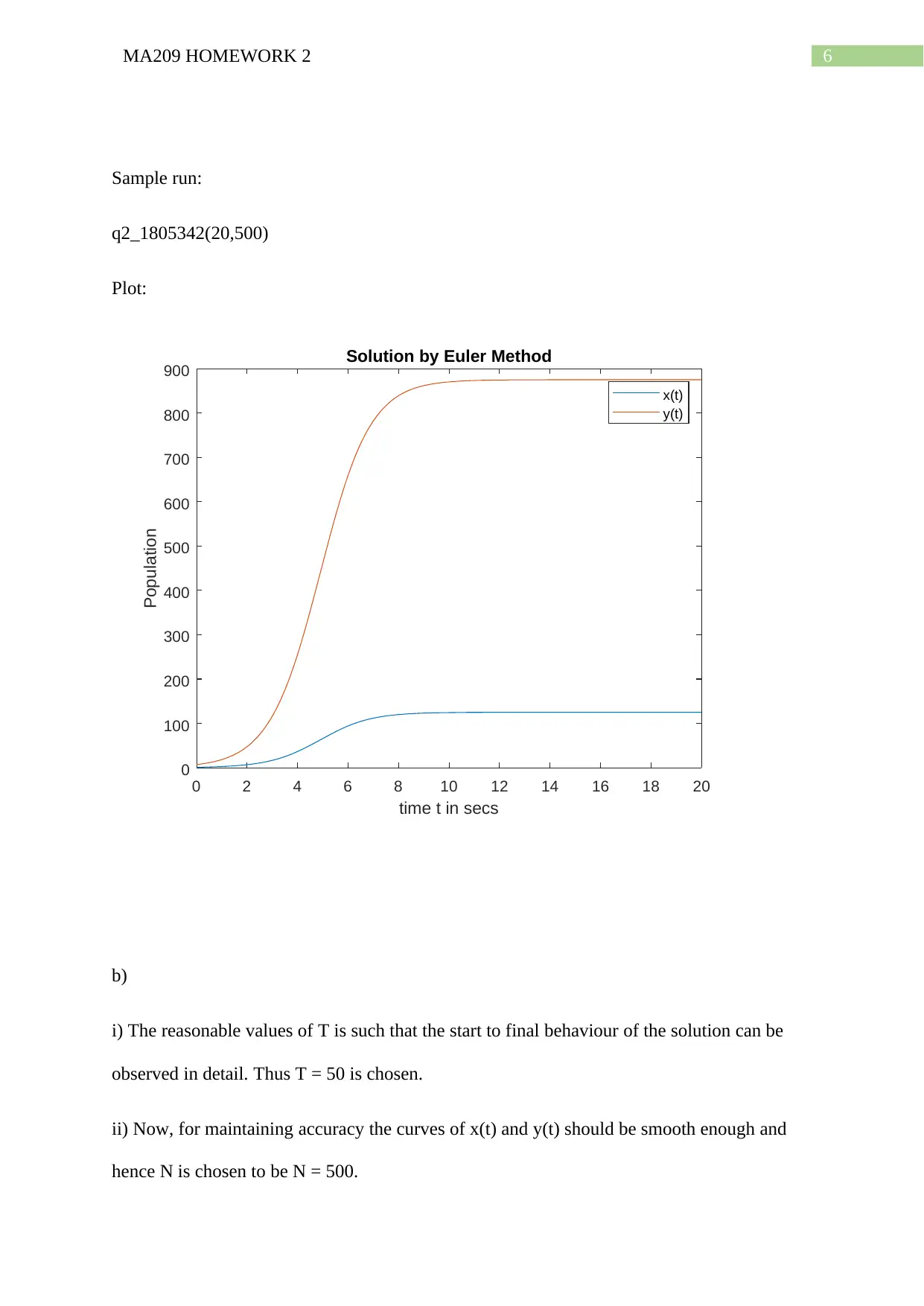
Sample run:
q2_1805342(20,500)
Plot:
0 2 4 6 8 10 12 14 16 18 20
time t in secs
0
100
200
300
400
500
600
700
800
900
Population
Solution by Euler Method
x(t)
y(t)
b)
i) The reasonable values of T is such that the start to final behaviour of the solution can be
observed in detail. Thus T = 50 is chosen.
ii) Now, for maintaining accuracy the curves of x(t) and y(t) should be smooth enough and
hence N is chosen to be N = 500.
Paraphrase This Document
Need a fresh take? Get an instant paraphrase of this document with our AI Paraphraser
7MA209 HOMEWORK 2
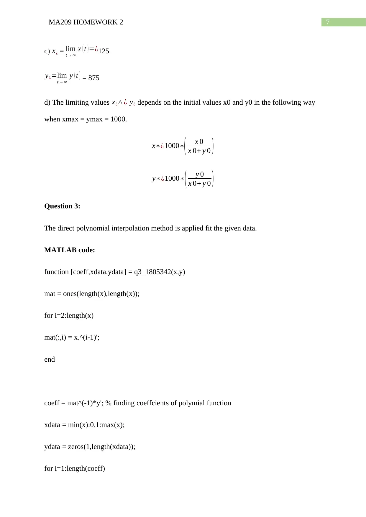
c) x¿ = lim
t → ∞
x ( t )=¿125
y¿=lim
t → ∞
y ( t ) = 875
d) The limiting values x¿∧¿ y¿ depends on the initial values x0 and y0 in the following way
when xmax = ymax = 1000.
x∗¿ 1000∗( x 0
x 0+ y 0 )
y∗¿1000∗( y 0
x 0+ y 0 )
Question 3:
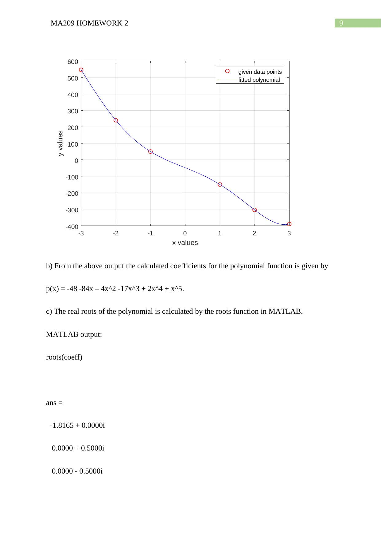
The direct polynomial interpolation method is applied fit the given data.
MATLAB code:
function [coeff,xdata,ydata] = q3_1805342(x,y)
mat = ones(length(x),length(x));
for i=2:length(x)
mat(:,i) = x.^(i-1)';
end
coeff = mat^(-1)*y'; % finding coeffcients of polymial function
xdata = min(x):0.1:max(x);
ydata = zeros(1,length(xdata));
for i=1:length(coeff)
8MA209 HOMEWORK 2
ydata = ydata + coeff(i).*xdata.^(i-1); % evaluating polymial at x points
end
plot(x,y,'ro',xdata,ydata,'b-')
grid on
xlabel('x values')
ylabel('y values')
legend('given data points','fitted polynomial')
end
Output:
>> x = [-3,-2,-1,1,2,3];
>> y = [546,240,50,-150,-304,-390];
>> q3_1805342(x,y)
ans =
-48.0000
-84.0000
-4.0000
-17.0000
2.0000
1.0000
Plot:
⊘ This is a preview!⊘
Do you want full access?
Subscribe today to unlock all pages.

Trusted by 1+ million students worldwide
9MA209 HOMEWORK 2
-3 -2 -1 0 1 2 3
x values
-400
-300
-200
-100
0
100
200
300
400
500
600
y values
given data points
fitted polynomial
b) From the above output the calculated coefficients for the polynomial function is given by
p(x) = -48 -84x – 4x^2 -17x^3 + 2x^4 + x^5.
c) The real roots of the polynomial is calculated by the roots function in MATLAB.
MATLAB output:
roots(coeff)
ans =
-1.8165 + 0.0000i
0.0000 + 0.5000i
0.0000 - 0.5000i
Paraphrase This Document
Need a fresh take? Get an instant paraphrase of this document with our AI Paraphraser

10MA209 HOMEWORK 2
0.2500 + 0.0000i
-0.1835 + 0.0000i
Hence, the real roots are x1 = -1.8165, x2 = 0.25, x3 = -0.1835.
0.2500 + 0.0000i
-0.1835 + 0.0000i
Hence, the real roots are x1 = -1.8165, x2 = 0.25, x3 = -0.1835.
1 out of 11
Related Documents
Your All-in-One AI-Powered Toolkit for Academic Success.
+13062052269
info@desklib.com
Available 24*7 on WhatsApp / Email
![[object Object]](/_next/static/media/star-bottom.7253800d.svg)
Unlock your academic potential
Copyright © 2020–2026 A2Z Services. All Rights Reserved. Developed and managed by ZUCOL.


