Machine Learning Algorithm PDF

TRACK DETECTION OF AESA RADAR USING HIGH END MACHINE
LEARNING ALGORITHM
Abstract:
Active Electronically Scanned Array (AESA) Radar is a development of solid state electronic
device in which each and every module broadcast its own independent signal. This particular
system has an excellent feature which is known as beam agility. With the help of this feature the
tracking could be done instantaneously for multiple targets for various azimuth angles. This
paper mainly focuses on the implementation of high-end machine learning that utilizes Support
Vector algorithm (SVM) to detect the track based on its classification.
Keywords: AESA, beam agility, azimuth angle, radar, Machine learning, Support Vector
algorithm (SVM)
Introduction:
Active Electronically Scanned Array (AESA) Radar is an advanced technology that is currently
in advancement. Both the AESA and PESA (passive) radar consists of numerous antennas and
transmitter. The main variation between the AESA and PESA (Passive) radar is that AESA radar
could generate its own microwave signal with its altering phase, i.e., it could be able to change
its angle position (from one azimuth angle to another) [1]. They could be able to operate at
varied frequencies (around 1000 frequency in a second). The major problem arises here is
occurrence of false alarm due to the sensor indication [2]. This could be caused due to the certain
unwanted object that could fall on the track giving a disturbance to the object of interest. Certain
measures could be taken to control it. We know that machine learning algorithm have raised its
head into every new invention and technologies since it could make a machine to learn by its
own [3] [4]. In this paper the particular detection of track and the classification of the track using
machine learning algorithm is explained.
Technical overview:
AESA radar is widely used in various fields especially for the military purposes. In our approach
we’re going to concentrate only on Support Vector Machines (SVM). SVM is nothing but a
classification algorithm [5]. Here, for the detection of the track we could use various sensors that
could follow the principle of micro-Doppler’s effect. Second the track detected should be
classified based on the high-end machine learning algorithm. Normally classification could be
done based on the statistics. Then these statistical data should be compared. Comparison and the
classification could be either discriminative or generative [6]. The adequacy of SVM could be
used for this purpose.
Support Vector Machines (SVM):

SVMs are one of the supervised learning models in machine learning same employed for
analysis. In SVM model the training/test samples are represented as dot/points in the space and
they are mapped in such a way that the clear gap among the categories appears which separates
the samples [7]. New test samples/examples are later mapped on the Using the kernel trick
SVMs are also be able to perform non-linear classification in addition to linear classification.
SVMs automatically map the inputs with high dimensional feature/attribute spaces. In general
SVM supports to construct hyper plane in any space and this can be employed for any tasks such
as regression, prediction or classification. SVM hyper plane is the only responsible for good
separation of training data with the largest distance to its nearby data [8]. This approach is
generally known as functional margin [9]. The state of the rule is if margin is larger than the
generalization error of classifier will be lower.
The main aim of ordering the tracks is to exactly forecast the target class from the data in each
case. The classifier engine process includes two steps:
1. Classifier Building: This method is to build a learning phase. The classifier, which evolved
from training certain databases instances/tuples, is constructed by the classification algorithms.
Individual instance/tuples that is composed of the preparation group is mentioned as a group.
These tuples can also be mentioned to as data points.
2. Usage of Classifier – The training model/classifier generated employing the data set will
classify test data set objects/tuples.
• Relevance Analysis: Database could consist of some unrelated attributes. Correlation analysis
will identify any two given attributes are associated.
• Data Transformation and lessening: The following methods help in data transformation:
– Normalization: This transformation occupies scaling every value that will make them descend
within a specific range [10] [11] [12]. This method is mainly used in the learning step when the
neural networks or the methods evolving measurements are employed.
– Simplification: This is a major concept of transforming. Here we can use the hierarchy
concept.
If the detected tracks of n points is given and the method of it is (−x→1 , y1 ) ........ (−x→n , yn )
and here yi is 1, this indicates the class with the sample →−xi is present. Each →−xi is a real
vector of p-dimension [13]. Our interest is detecting the “extreme- margin hyper plane” which
separates the category of samples from →−xi. This is required to be definite to maximize the
distance among the hyper plane as well as the adjacent sample →−xi.

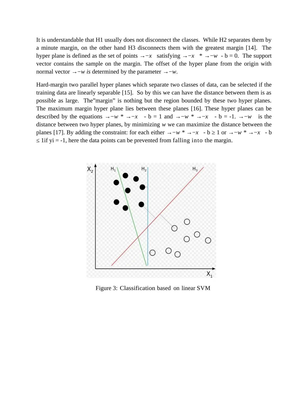
It is understandable that H1 usually does not disconnect the classes. While H2 separates them by
a minute margin, on the other hand H3 disconnects them with the greatest margin [14]. The
hyper plane is defined as the set of points →−x satisfying →−x * →−w - b = 0. The support
vector contains the sample on the margin. The offset of the hyper plane from the origin with
normal vector →−w is determined by the parameter →−w.
Hard-margin two parallel hyper planes which separate two classes of data, can be selected if the
training data are linearly separable [15]. So by this we can have the distance between them is as
possible as large. The”margin” is nothing but the region bounded by these two hyper planes.
The maximum margin hyper plane lies between these planes [16]. These hyper planes can be
described by the equations →−w * →−x - b = 1 and →−w * →−x - b = -1. →−w is the
distance between two hyper planes, by minimizing w we can maximize the distance between the
planes [17]. By adding the constraint: for each either →−w * →−x - b ≥ 1 or →−w * →−x - b
≤ 1if yi = -1, here the data points can be prevented from falling into the margin .
Figure 3: Classification based on linear SVM

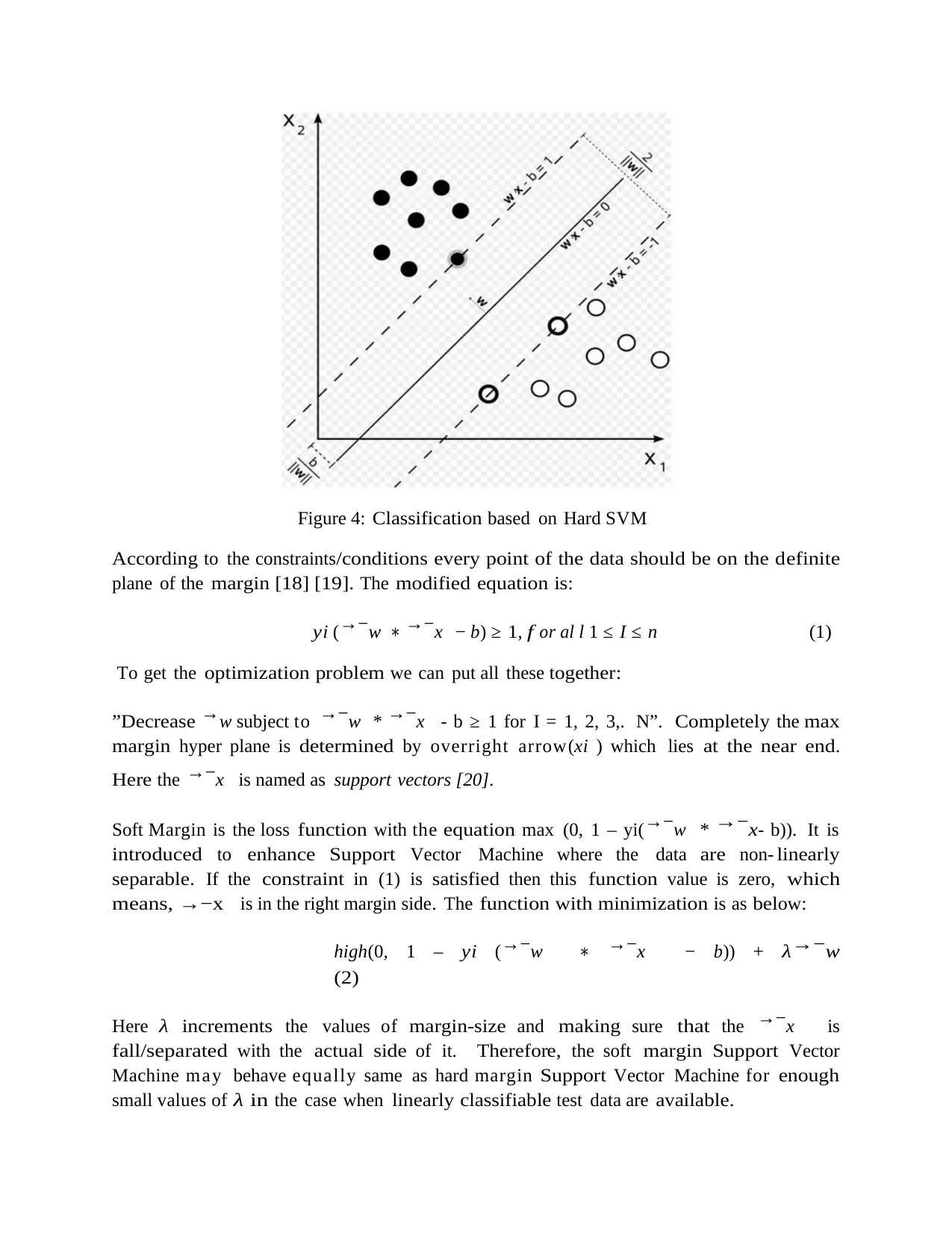
Figure 4: Classification based on Hard SVM
According to the constraints /conditions every point of the data should be on the d efinite
plane of the margin [18] [19]. The modified equation is :
y i (→−w ∗ →−x − b) ≥ 1 , f o r al l 1 ≤ I ≤ n (1)
To get the optimization problem we can put all these together:
”Decrease →w subject to →−w * →−x - b ≥ 1 for I = 1, 2, 3,. N”. Completely the max
margin hyper plane is determined by overright arrow(xi ) which lies at the near end.
Here the →−x is named as support vectors [20] .
Soft Margin is the loss function with the equation max (0, 1 – yi(→−w * → −x- b)). It is
introduced to enhance Support Vector Machine where the data are non- linearly
separable. If the constraint in (1) is satisfied then this function value is zero, which
means, →−x is in the right margin side . The function with minimization is as bel ow:
high(0, 1 – y i (→−w ∗ →−x − b)) + λ→−w
(2)
Here λ increments the values of margin-size and making sure that the →−x is
fall/separated with the actual side of it. Therefore, the soft margin Support Vector
Machine may behave equally same as hard margin Support Vector Machine for enough
small values of λ in the case when linearly classifiable test data are av ailable.

Evaluation:
Here we employ feature vector in order to detect the tracks [21] [22]. The tracks are
detected by the radar range equation given below.
R= (Gt Gr P1 λ2 σ |(4 π )3 K T 0 BF( SNR)min L )1/ 4
(3)
Where,
G t, Gr - Transceiver Gain
P 1 – power transmitted
Σ – radar cross section
(SNR) min – Minimum signal to noise ratio
L - System loss factor
No
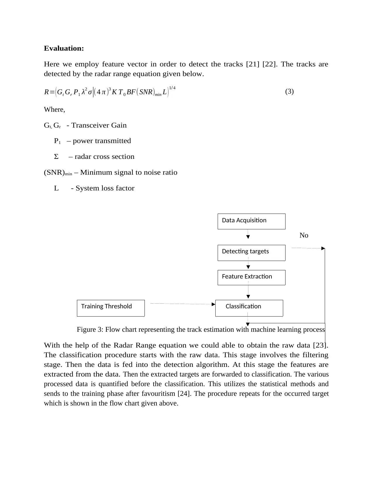
Figure 3: Flow chart representing the track estimation with machine learning process
With the help of the Radar Range equation we could able to obtain the raw data [23].
The classification procedure starts with the raw data. This stage involves the filtering
stage. Then the data is fed into the detection algorithm. At this stage the features are
extracted from the data. Then the extracted targets are forwarded to classification. The various
processed data is quantified before the classification. This utilizes the statistical methods and
sends to the training phase after favouritism [24]. The procedure repeats for the occurred target
which is shown in the flow chart given above.
Detecting targets
Data Acquisition
Feature Extraction
ClassificationTraining Threshold

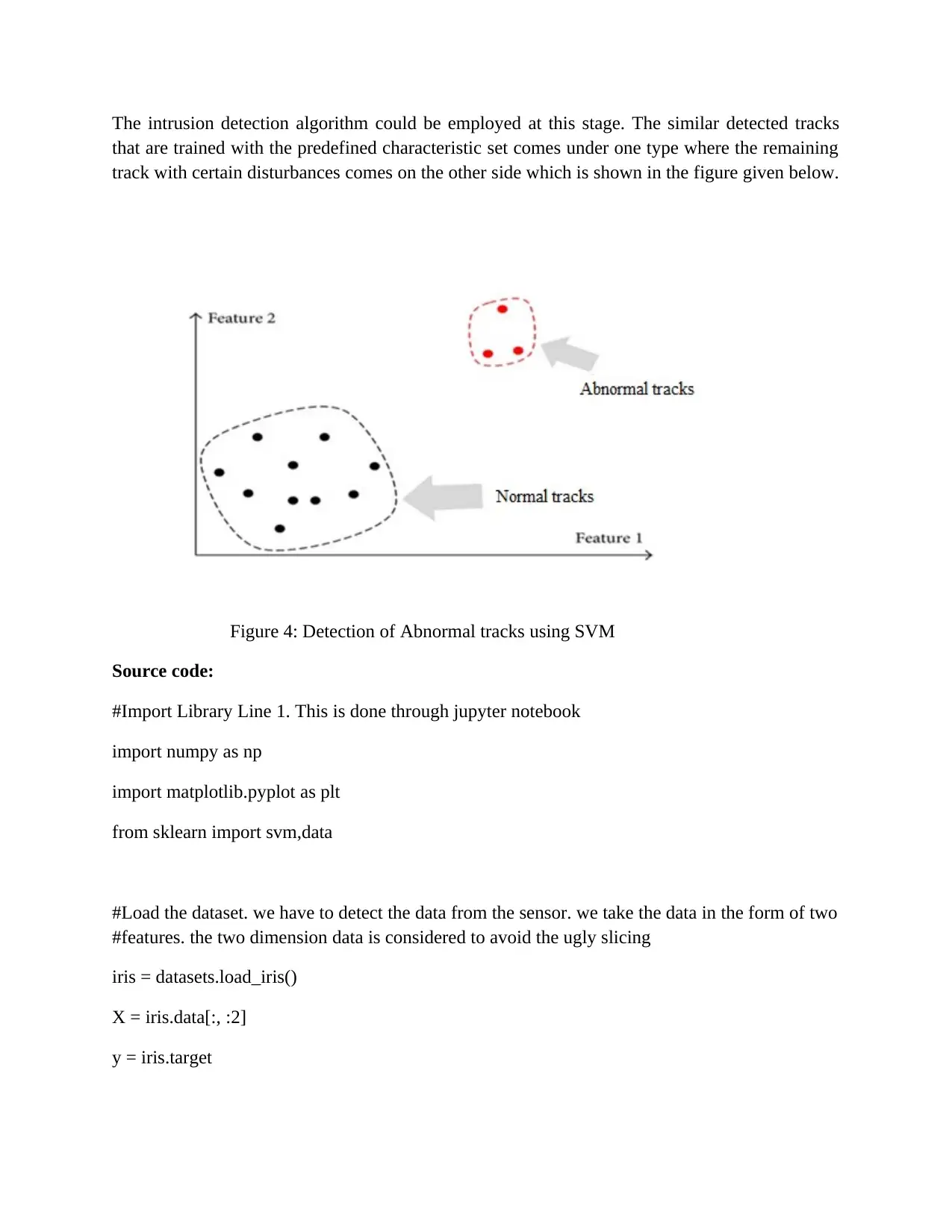
The intrusion detection algorithm could be employed at this stage. The similar detected tracks
that are trained with the predefined characteristic set comes under one type where the remaining
track with certain disturbances comes on the other side which is shown in the figure given below.
Figure 4: Detection of Abnormal tracks using SVM
Source code:
#Import Library Line 1. This is done through jupyter notebook
import numpy as np
import matplotlib.pyplot as plt
from sklearn import svm,data
#Load the dataset. we have to detect the data from the sensor. we take the data in the form of two
#features. the two dimension data is considered to avoid the ugly slicing
iris = datasets.load_iris()
X = iris.data[:, :2]
y = iris.target

# Line 3. Plot the map
from sklearn import make_blobs
(X,y) = make_blobs(n_samples=50,n_features=2,centers=2,cluster_std=1.05,random_state=40)
#we need to add 1 to X values (we can say its bias)
XX = np.c_[np.ones((X.shape[0])),X]
plt.xlabel('Feature 1')
plt.ylabel('Feature 2')
plt.scatter(XX[:,1],XX[:,2],marker='o',c=r)# default marker is 'o'
plt.axis([-4,12,-10,-2])
plt.show()
Conclusion:
Through our paper we have generated a solution to ignore the abnormal track and take the
necessary track using high end machine learning algorithm. The advantages of AESA radar
technology are many. These technologies are highly adapted in the field of air and naval forces
that uses AESA radar to detect minute targets at a wider range. Electronic surveillance system
finds difficult to vary in its frequencies for detecting the position. But AESA could highly vary
in its frequencies with a minute pulse at a random sequence. The greatest advantage is to resist
jammers. But a minor disadvantage is that since it could show variations in its frequencies, this
system could no longer persist in its life time.
References:
[1] Y. Yinan, L. Jiajin, Z. Wenxue, and L. Chao, "Target classification and pattern recognition
using micro-Doppler radar signatures," in Software Engineering, Artificial Intelligence,
Networking, and Parallel/Distributed Computing, Seventh ACIS International Conference on,
2006, pp. 213-217.
[2] Tom Jeffrey , “ Phased Array Radar Design : Application Of Radar Fundamentals ”, Scitech
Publishing Inc,2009
[3] R. Zekavat and R. Buehrer, Wireless Localization Using Ultra-Wideband Signals, 1st ed.
Wiley-IEEE Press, 2012.

[4] J. P. Haftbaradaran,M. Kamarei, and R.F.Mofrad. “The optimal search for multifunction
phased array radar”. In Antennas Propagation Conference, 2009. LAPC 2009. Loughborough,
pages 609 –612, nov. 2009
[5] M. Chiani and A. Giorgetti, “Coexistence between UWB and narrowband wireless
communication systems,” Proc. IEEE, vol. 97, no. 2, pp. 231–254, Feb. 2009.
[6] M. Svecov ˇ a, D. Kocur, R. Zetik, and J. Rov ´ nˇakov ´ a, “Target localization ´ by a
multistatic UWB radar,” in Proc. 20th Int. Conf. Radioelektronika, Apr. 2010, pp. 1–4.
[7] Z. Xiao-wei, A. Gaugue, C. Liebe, J. Khamlichi, and M. M ` enard, ´ “Through the wall
detection and localization of a moving target with a bistatic UWB radar system,” in Proc.
European Radar Conf., Sep. 2010, pp. 204–207.
[8] S. Gezici, T. Zhi, G. Giannakis, H. Kobayashi, A. Molisch, H. Poor, and Z. Sahinoglu,
“Localization via ultra-wideband radios: a look at positioning aspects for future sensor
networks,” IEEE Signal Process. Mag., vol. 22, no. 4, pp. 70–84, Jul. 2005.
[9] G. E. Smith, K. Woodbridge, and C. J. Baker, "Micro-Doppler signature classification," in
Radar, 2006. CIE '06. International Conference on, 2006, pp. 1-4.
[10] K. Dae-Hyun, L. Dong-Woo, S. L. K. Hyung-Myung, W. Sung-Chul, and K. Y. Hyun,
“Localization methods of multi-targets for UWB radar sensor networks,” in Proc. Int. Asia-Pac.
Conf. on Synth. Aperture Radar, Sep. 2011, pp. 1–4.
[11] D. Hong, C. Chen, P. Shirui, L. Xin, and Z. Linhua, “Multistatic ultrawideband localization
for NLOS environments,” in Proc. Int. Conf. Intelligent Sys. Design Eng. App., Jan. 2012, pp.
380–384.
[12] H. Yuan, T. Savelyev, and A. Yarovoy, “Two-stage algorithm for extended target tracking
by multistatic UWB radar,” in Proc. IEEE CIE Int. Conf. Radar, vol. 1, Oct. 2011, pp. 795–799.
[13] M. Arulampalam, S. Maskell, N. Gordon, and T. Clapp, “A tutorial on particle filters for
online nonlinear/non-Gaussian Bayesian tracking,” IEEE Trans. Signal Process., vol. 50, no. 2,
pp. 174–188, Feb. 2002.
[14] T. Kai, W. Shiyou, C. Jie, L. Xiaojun, and F. Guangyou, “An efficient and low-complexity
through wall moving target tracking algorithm by UWB radar,” in Proc. 14th Int. Conf. Ground
Penetrating Radar, Jun. 2012, pp. 966–971.
[15] I. Bilik, J. Tabrikian, and A. Cohen, "GMM-based target classification for ground
surveillance Doppler radar," Aerospace and Electronic Systems, IEEE Transactions on, vol. 42,
pp. 267-278, January 2006.

[16] M. Chiani, A. Giorgetti, M. Mazzotti, R. Minutolo, and E. Paolini, “Target detection
metrics and tracking for UWB radar sensor networks,” in Proc. IEEE Int. Conf. Ultra-Wideband,
Sep. 2009, pp. 469–474.
[17] B. Sobhani, E. Paolini, A. Giorgetti, M. Mazzotti, and M. Chiani, “Target tracking for UWB
multistatic radar sensor networks,” IEEE J. Sel. Topics Signal Process., vol. 8, no. 1, pp. 125–
136, Feb. 2014.
[18] B. Sobhani, M. Mazzotti, E. Paolini, A. Giorgetti, and M. Chiani, “Effect of state space
partitioning on bayesian tracking for UWB radar sensor networks,” in Proc. IEEE Int. Conf.
Ultra-Wideband, Sep. 2013, pp. 120–125.
[19] E. Paolini, A. Giorgetti, M. Chiani, R. Minutolo, and M. Montanari, “Localization
capability of cooperative anti-intruder radar systems,” EURASIP J. Advances Signal Process.,
vol. 2008, pp. 1–14, 2008, article ID 726854.
[20] A. Giorgetti and M. Chiani, “Time-of-arrival estimation based on information theoretic
criteria,” IEEE Trans. Signal Process., vol. 61, no. 8, pp. 1869–1879, 2013.
[21] B. Sobhani, M. Mazzotti, E. Paolini, A. Giorgetti, and M. Chiani, “Multiple target detection
and localization in UWB multistatic radars,” in Proc. IEEE Int. Conf. Ultra-WideBand, Sep.
2014, pp. 135–140.
[22] S. Blackman, “Multiple hypothesis tracking for multiple target tracking,” IEEE Aerosp.
Electron. Syst. Mag., vol. 19, no. 1, pp. 5–18, 2004.
[23] H. Godrich, V. M. Chiriac, A. M. Haimovich and R. S. Blum, “Target tracking in MIMO
radar systems: Techniques and performance analysis,” in in Proc. IEEE Radar Conf.,
Washington, DC, pp. 1111-1116, May. 2010.
[24] M. Otero, "Application of a continuous wave radar for human gait recognition," in Signal
Processing, Sensor Fusion, and Target Recognition XIV, Proceedings of SPIE, Orlando, FL,
USA, 2005, pp. 538-548.