Machine Learning Application: Data Science Practice

This document explores the principles underlying several machine learning methods and their application in determining the price category of mobile phones. It covers topics such as machine learning pipelines, collaborative filtering, logistic regression, and K-means clustering. The document provides an introduction, objective, key system concepts, application of pipelines, collaborative filtering, logistic regression, and K-means, and a conclusion. It also includes references and an appendix with code snippets.

Title: Data Science Practice
Task: Machine Learning Application Using PySpark
Lecturer:
School:
Course Name:
Unit Code:
Due Date:

Machine Learning Application
1. Introduction
Several factors have been posited to affect the quality of manufactured goods. However, the
effect of specification when it comes to pricing of technological products goes a long way to
define every aspect related to the manufacturing of these technological items such as: phones,
software, personal computers, etcetera.
In practice, factors such as the quality of a phone’s camera, the bandwidth of its connectivity,
and battery life alongside other factors have been theorized to influence the price category that
a phone falls in. Nevertheless, it is prudent that both the customer and the manufacturer get
value for the product in focus. In line with this view, to achieve optimal value for both sides,
methods such as data mining and machine learning can be used to enable the determination of
the best price category that a phone falls in.
1.1 Objective
The objective of this study is to conduct an evaluation of the principles underlying several
machine learning methods.
2. Key System Concepts
2.1 Machine learning pipelines
To understand the concept of pipelines in machine learning (ML) practice, it is important that
we begin with the objective of MLs according to (Koen, 2018) i.e.:
i. Reduction of latency
ii. Fairly integrated with sufficient coupling to other ML system parts such as the GUI, data
storage etc.
iii. Ability to be scaled
iv. Message driven
Ideally, pipelines involve collection of data, “…sending it through an enterprise message bus
and processing it to provide pre-calculated results and guidance for next day’s operations”
(Koen, 2018). Pipelines therefore comprise of two straight forward components which include,
Online Model Analytics and Offline Data Discovery.
2.1.1 Application of Pipelines to the original ML project
From the process of data ingestion using PySpark which ensured that the dataset is processed
differently from the rest of the code so as to utilize the functionality of multiple server cores
and processors which are provided in the documentation of PySpark. Our application of
pipelines included data extraction, feature transformation, and feature selection.
2.2 Collaborative filtering
In machine learning, Collaborative filtering (CF) is among the most applied techniques when it
comes recommender systems (Ricci, et al., 2011). It generally has two senses i.e., a narrow one
and a more general one. From a narrower sense, a CF is used in defining processes that enable
automatic predictions (filtering). In this view, the assumptions that underlay the CF is that, in
the event that “…a person A has the same opinion as a person B on an issue, A is more likely to
2
Name:

Machine Learning Application
have B's opinion on a different issue than that of a randomly chosen person” (Wayback
Machine, 2012).
2.2.1 Application of CF
The application of CF in this study involved the adoption of an Alternative Least Squares (ALS)
Algorithm which is traditionally used to decompose large matrix to a lower dimensional user
factors and item factors. The advantages of ALS lie in its ability to provide an alternative
approach to optimizing the loss function (Koehler, 2017). After the application of data and
model training, we conducted prediction using the ALS model to aid in the prediction of the
price category in which a mobile phone can be classified.
2.3 Logistic Regression (LR)
Unlike linear regression models whose dependent variable is often a continuous, logistic
regression models are used in the prediction of nominal response variables that have two or
more categories. In modern parlance practices, LR “…is viewed as a generalized linear model.
The parameters for the best fit model are estimated using maximum likelihood rather than
least squares” (Dransfield & Phil, 2013). As such, the implementation of LR models often takes
two paths, i.e. the unconditional approach and the conditional approach whereby the
unconditional approach suffices in cases where the number of degrees of freedom of a given
model is relatively small compared to the number of observations.
2.3.1 Application of LR
However, in cases where there are larger degrees of freedom, it is important that the
conditional approach must be used as in our case where the number of observations were
approximately 3000.
In application, we applied a logistic regression using a PySpark library on training a model with
2129 observations as a training set and 871 observations as the test set. Moreover, to test the
performance of the LR model, we examined the area under curve alongside the model’s
prediction accuracy.
2.4 K-Means
Categorized under unsupervised learning algorithms, the K-Means is implemented as a
clustering model which follows a simple approach i.e.: through the assumption k clusters fixed
Apriori, the algorithm follows the principle of defining k centers which are allocated to every
cluster. To improve performance of the model, the centers are placed far away from each other
as possible. After which each point of the data is associated it to the nearest center. Generally,
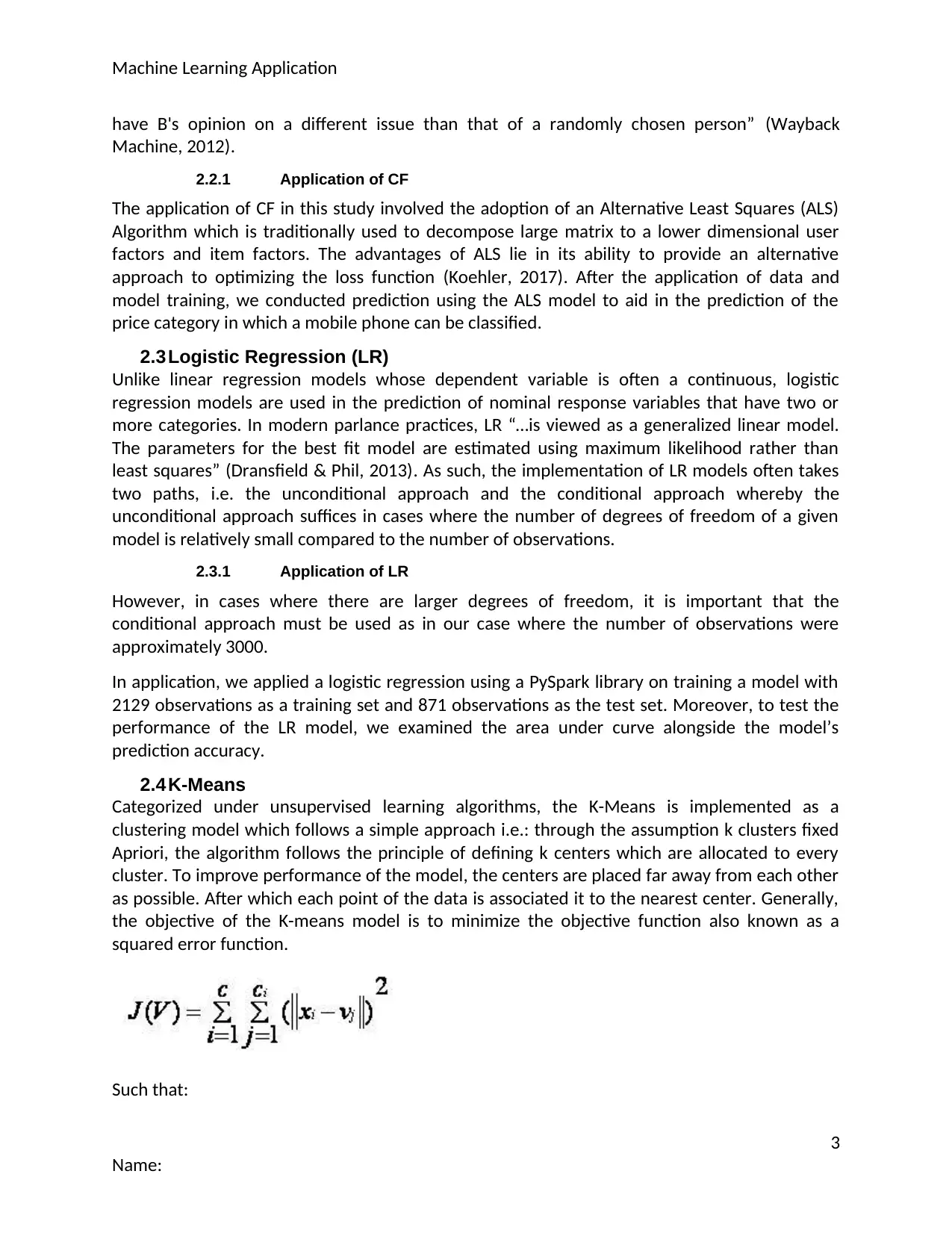
the objective of the K-means model is to minimize the objective function also known as a
squared error function.
Such that:
3
Name:

Machine Learning Application
||xi - vj|| is the Euclidean distance between xi and vj, ci is the number of data points in ith cluster,
and c is the number of cluster centers.
2.4.1 Application of K-Means
In our study, we applied the Knn model with 3 initial clusters on the data “features which we
had defined earlier during pipeline development and data transformation. The evaluation of the
model’s performance was examined using the Squared Errors and squared Euclidean distance.
3. Conclusion
Machine learning is a relatively extensive concept in the modern era of data integration into
real life. From Artificial intelligence, Business intelligence, medical application and many other
fields, the application of ML is crucial in enabling both organizations and individuals reach the
vast benefits offered by data. Despite all the potential in ML, determination of the best model
that can be applied to a given set of data is still a concern a fact that often prompts the
application of a number of models from which the optimum is examined and chosen as in our
case.
In conclusion, it is therefore crucial that the right preliminary steps are adopted and the correct
methods for the application of ML algorithms are used if an organization is to benefit from the
concept of machine learning.
4
Name:

Machine Learning Application
4. References
Dransfield, B. & Phil, D., 2013. Avoiding and Detecting Statistical Malpractice (Design & Analysis
for Biologists, with R). 3rd ed. Bristol: InfluentialPoints.
Koehler, V., 2017. ALS Implicit Collaborative Filtering. [Online]
Available at: https://medium.com/radon-dev/als-implicit-collaborative-filtering-5ed653ba39fe
[Accessed 13 June 2019].
Koen, S., 2018. Architecting a Machine Learning Pipeline. [Online]
Available at: https://towardsdatascience.com/architecting-a-machine-learning-pipeline-
a847f094d1c7
[Accessed 13 June 2019].
Ricci, F., Rokach, L. & Shapira, B., 2011. Introduction to Recommender Systems Handbook. 1st
ed. Washington: Springer.
Wayback Machine, 2012. An integrated approach to TV & VOD Recommendations. [Online]
Available at: http://www.redbeemedia.com/insights/integrated-approach-tv-vod-
recommendations
[Accessed 13 June 2019].
Appendix
# coding: utf-8
# In[3]:
import os
import pyspark
os.environ["JAVA_HOME"] = "c:\java"
os.environ["SPARK_HOME"] = "e:\spark\spark-2.4.3-bin-hadoop2.7"
import findspark
findspark.init()
from pyspark.sql import SparkSession
# In[4]:
#Importing the Economic factors data
5
Name:

Machine Learning Application
spark = SparkSession.builder.appName('Economic-factors').getOrCreate()
# ###### The objective of this analysis is to determine the factors that best influence
determination of the price range in which a manufactured mobile falls.
# The dataset used is obtained from https://www.kaggle.com/iabhishekofficial/mobile-price-
classification/downloads/mobile-price-classification.zip/1 where it was initially split into
training and test sets. However, for use in this study, the two datasets are initially combined in
such a way that the first 2000 observation consists of the training data and the subsequent
1000 observations comprise the test data so as to ease the process of importing into the
pyspark environment. During classification and prediction analysis, the data will be split
according to the original ratio
# ### Getting the data
# In[22]:
data = spark.read.csv('mobile-price-classification.csv', header = True)
train=spark.read.csv('train.csv', header = True)
test=spark.read.csv('test.csv', header = True)
# ### Task 1.1: Exploratory data analysis
# #### Number of rows and columns
# In[6]:
#Examining the variables contained in the data
data.printSchema()
# In[7]:
data.show(10)
# In[8]:
train.show(10)
# In[9]:
test.show(10)
# #### Number of rows
# In[10]:
data.count()
# #### Number of Columns
# In[11]:
6
Name:

Machine Learning Application
len(data.columns)
# In[12]:
import pandas as pd
dataa=pd.DataFrame(data.take(3000), columns=data.columns)
# ### Cleaning data
# #### Removing missing observations
# There are no missing observations in the dataset since the data is recorded by a computer
during production. Furthermore, the data was cleaned at the source by the data provider
# ### Summarizing data through plotting
# #### Plotting Price range, Talk Time, and Internal memory
# ##### Price range
# In[13]:
#Creating a dataframe for use in ploting
import matplotlib.pyplot as plt
# In[34]:
plt.style.use('ggplot')
Price_Range='0','1','2','3'
sizes = [215, 130, 245, 210]
colors = ['gold', 'yellowgreen', 'lightcoral', 'lightskyblue']
explode = (0.1, 0, 0, 0)
Price=dataa["price_range"].value_counts()
plt.pie(Price,autopct='%1.1f%%',explode=explode, labels=Price_Range, shadow=False,
startangle=140)
plt.title('Percentage Distribution of the Price range of the manufactured Phones')
# ##### Talk Time
# In[33]:
plt.style.use('classic')
talk_time = dataa["talk_time"]
talk_time=talk_time.value_counts()
7
Name:

Machine Learning Application
talk_time=list(talk_time)
plt.hist(talk_time, bins=12)
plt.grid(axis='y', alpha=0.75)
plt.xlabel('Talk Time')
plt.ylabel('Frequency')
plt.title('Distribution of the Talk time in the manufactured phones')
# ##### Internal memory
# In[14]:
internalmemory = dataa['int_memory']
plt.style.use('classic')
talk_time=internalmemory.value_counts()
talk_time=list(talk_time)
plt.hist(talk_time, bins=12)
plt.grid(axis='y', alpha=0.75)
plt.xlabel("Internal Memory")
plt.ylabel("Size")
plt.title("Distribution of the size of internal memory in the manufactured phones")
# ## Task I.2: Recommendation engine
# ### Model Training
# In[26]:
data = spark.read.csv('mobile-price-classification.csv', header = True)
from pyspark.ml.recommendation import ALS
from pyspark.ml.evaluation import RegressionEvaluator
training, test = data.randomSplit([0.8,0.2])
data.show(
# #### Alternative Least Squares Algorithm
# In[27]:
### Model Predictions
8
Name:

Machine Learning Application
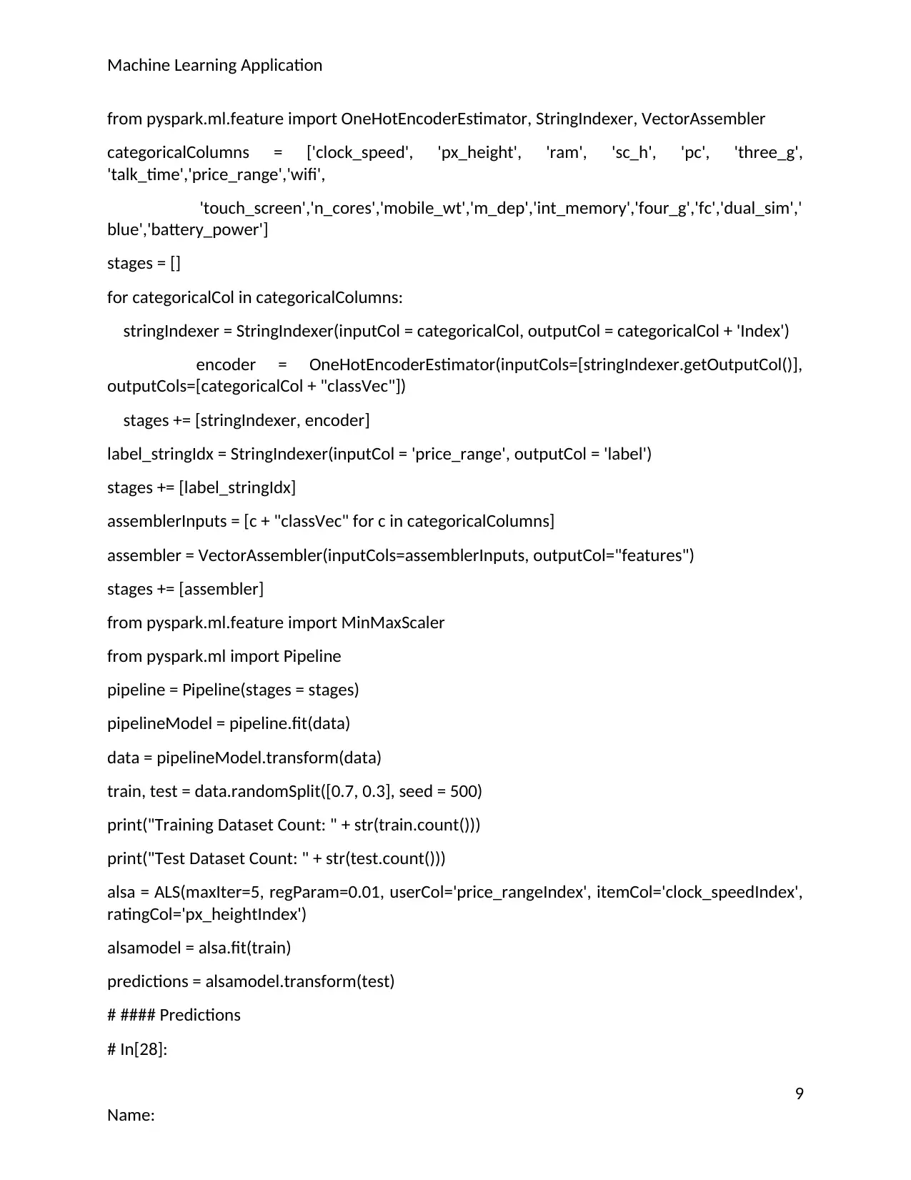
from pyspark.ml.feature import OneHotEncoderEstimator, StringIndexer, VectorAssembler
categoricalColumns = ['clock_speed', 'px_height', 'ram', 'sc_h', 'pc', 'three_g',
'talk_time','price_range','wifi',
'touch_screen','n_cores','mobile_wt','m_dep','int_memory','four_g','fc','dual_sim','
blue','battery_power']
stages = []
for categoricalCol in categoricalColumns:
stringIndexer = StringIndexer(inputCol = categoricalCol, outputCol = categoricalCol + 'Index')
encoder = OneHotEncoderEstimator(inputCols=[stringIndexer.getOutputCol()],
outputCols=[categoricalCol + "classVec"])
stages += [stringIndexer, encoder]
label_stringIdx = StringIndexer(inputCol = 'price_range', outputCol = 'label')
stages += [label_stringIdx]
assemblerInputs = [c + "classVec" for c in categoricalColumns]
assembler = VectorAssembler(inputCols=assemblerInputs, outputCol="features")
stages += [assembler]
from pyspark.ml.feature import MinMaxScaler
from pyspark.ml import Pipeline
pipeline = Pipeline(stages = stages)
pipelineModel = pipeline.fit(data)
data = pipelineModel.transform(data)
train, test = data.randomSplit([0.7, 0.3], seed = 500)
print("Training Dataset Count: " + str(train.count()))
print("Test Dataset Count: " + str(test.count()))
alsa = ALS(maxIter=5, regParam=0.01, userCol='price_rangeIndex', itemCol='clock_speedIndex',
ratingCol='px_heightIndex')
alsamodel = alsa.fit(train)
predictions = alsamodel.transform(test)
# #### Predictions
# In[28]:
9
Name:

Machine Learning Application
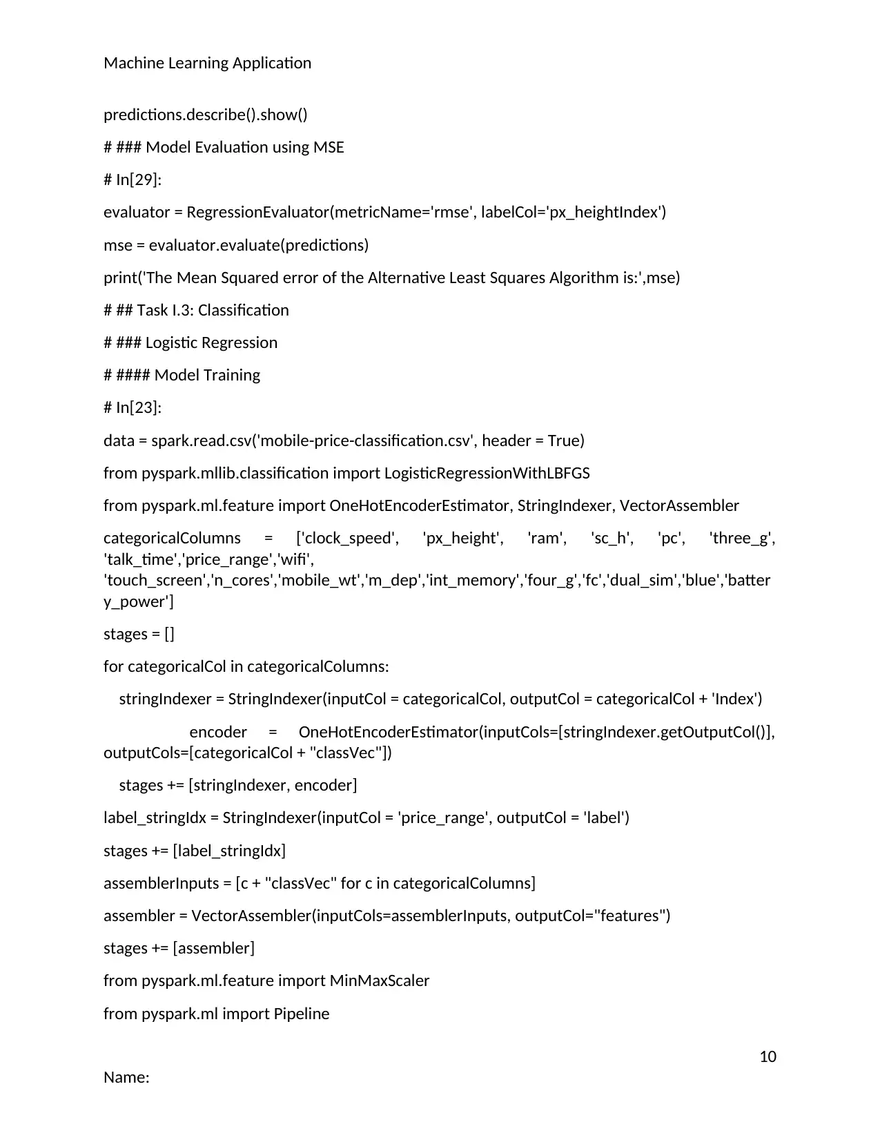
predictions.describe().show()
# ### Model Evaluation using MSE
# In[29]:
evaluator = RegressionEvaluator(metricName='rmse', labelCol='px_heightIndex')
mse = evaluator.evaluate(predictions)
print('The Mean Squared error of the Alternative Least Squares Algorithm is:',mse)
# ## Task I.3: Classification
# ### Logistic Regression
# #### Model Training
# In[23]:
data = spark.read.csv('mobile-price-classification.csv', header = True)
from pyspark.mllib.classification import LogisticRegressionWithLBFGS
from pyspark.ml.feature import OneHotEncoderEstimator, StringIndexer, VectorAssembler
categoricalColumns = ['clock_speed', 'px_height', 'ram', 'sc_h', 'pc', 'three_g',
'talk_time','price_range','wifi',
'touch_screen','n_cores','mobile_wt','m_dep','int_memory','four_g','fc','dual_sim','blue','batter
y_power']
stages = []
for categoricalCol in categoricalColumns:
stringIndexer = StringIndexer(inputCol = categoricalCol, outputCol = categoricalCol + 'Index')
encoder = OneHotEncoderEstimator(inputCols=[stringIndexer.getOutputCol()],
outputCols=[categoricalCol + "classVec"])
stages += [stringIndexer, encoder]
label_stringIdx = StringIndexer(inputCol = 'price_range', outputCol = 'label')
stages += [label_stringIdx]
assemblerInputs = [c + "classVec" for c in categoricalColumns]
assembler = VectorAssembler(inputCols=assemblerInputs, outputCol="features")
stages += [assembler]
from pyspark.ml.feature import MinMaxScaler
from pyspark.ml import Pipeline
10
Name:

Machine Learning Application
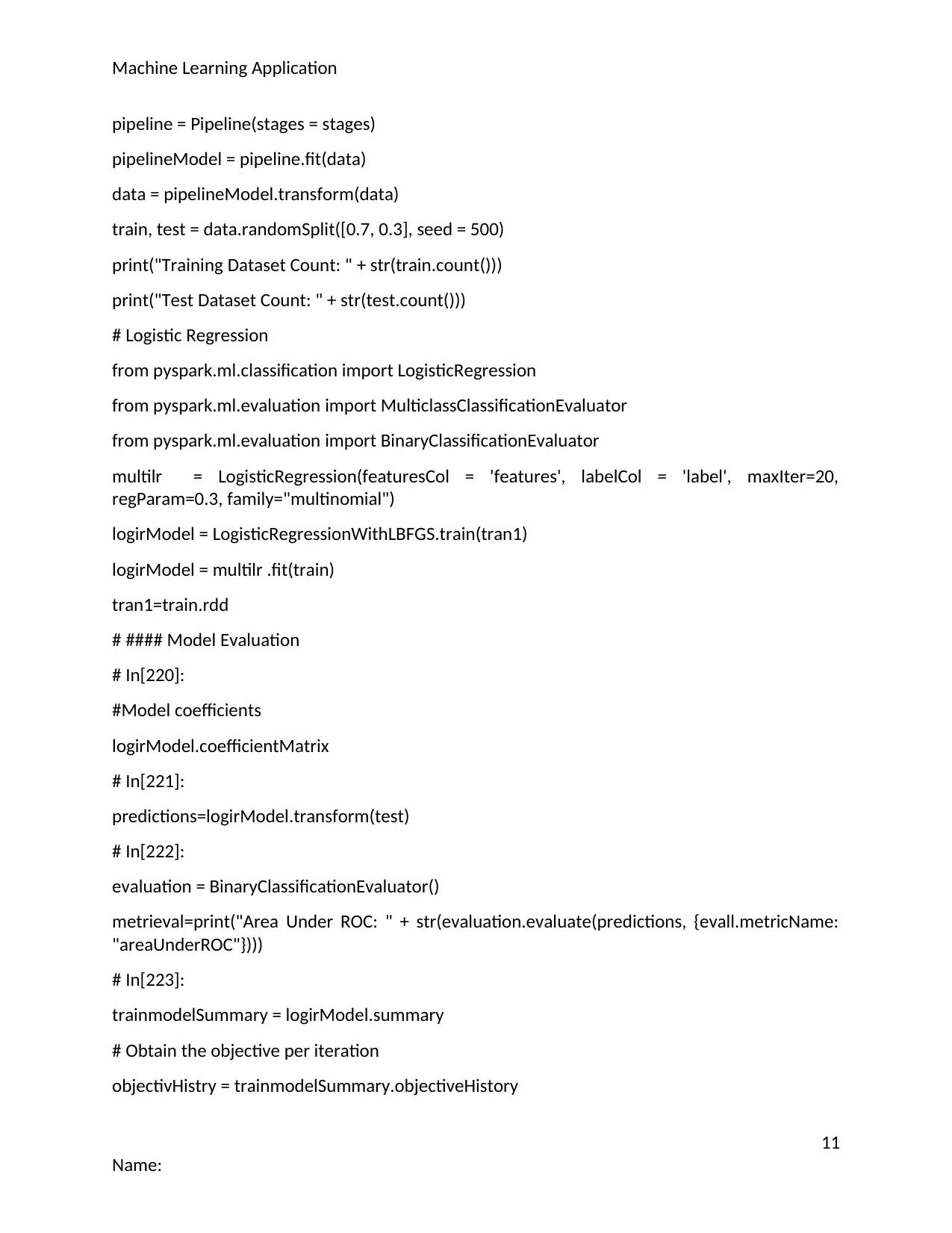
pipeline = Pipeline(stages = stages)
pipelineModel = pipeline.fit(data)
data = pipelineModel.transform(data)
train, test = data.randomSplit([0.7, 0.3], seed = 500)
print("Training Dataset Count: " + str(train.count()))
print("Test Dataset Count: " + str(test.count()))
# Logistic Regression
from pyspark.ml.classification import LogisticRegression
from pyspark.ml.evaluation import MulticlassClassificationEvaluator
from pyspark.ml.evaluation import BinaryClassificationEvaluator
multilr = LogisticRegression(featuresCol = 'features', labelCol = 'label', maxIter=20,
regParam=0.3, family="multinomial")
logirModel = LogisticRegressionWithLBFGS.train(tran1)
logirModel = multilr .fit(train)
tran1=train.rdd
# #### Model Evaluation
# In[220]:
#Model coefficients
logirModel.coefficientMatrix
# In[221]:
predictions=logirModel.transform(test)
# In[222]:
evaluation = BinaryClassificationEvaluator()
metrieval=print("Area Under ROC: " + str(evaluation.evaluate(predictions, {evall.metricName:
"areaUnderROC"})))
# In[223]:
trainmodelSummary = logirModel.summary
# Obtain the objective per iteration
objectivHistry = trainmodelSummary.objectiveHistory
11
Name:

Machine Learning Application
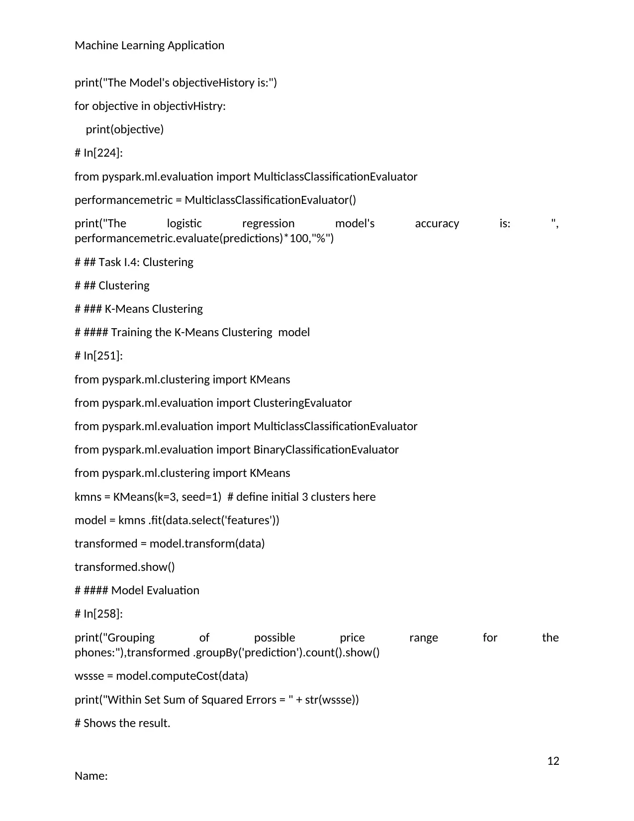
print("The Model's objectiveHistory is:")
for objective in objectivHistry:
print(objective)
# In[224]:
from pyspark.ml.evaluation import MulticlassClassificationEvaluator
performancemetric = MulticlassClassificationEvaluator()
print("The logistic regression model's accuracy is: ",
performancemetric.evaluate(predictions)*100,"%")
# ## Task I.4: Clustering
# ## Clustering
# ### K-Means Clustering
# #### Training the K-Means Clustering model
# In[251]:
from pyspark.ml.clustering import KMeans
from pyspark.ml.evaluation import ClusteringEvaluator
from pyspark.ml.evaluation import MulticlassClassificationEvaluator
from pyspark.ml.evaluation import BinaryClassificationEvaluator
from pyspark.ml.clustering import KMeans
kmns = KMeans(k=3, seed=1) # define initial 3 clusters here
model = kmns .fit(data.select('features'))
transformed = model.transform(data)
transformed.show()
# #### Model Evaluation
# In[258]:
print("Grouping of possible price range for the
phones:"),transformed .groupBy('prediction').count().show()
wssse = model.computeCost(data)
print("Within Set Sum of Squared Errors = " + str(wssse))
# Shows the result.
12
Name:

Machine Learning Application
centers = model.clusterCenters()
print("Cluster Centers: ")
for center in centers:
print(center)
preds1=model.transform(test)
evaluation = ClusteringEvaluator()
silhout = evaluation.evaluate(preds)
print("Silhouette with squared euclidean distance = " + str(silhout))
# ## Bibliography
# BEN KEEN.(2018). Bar Charts in Matplotlib. Retrieved From: http://benalexkeen.com/bar-
charts-in-matplotlib/
# Apache Spark. (2012). Working with Pyspark for Machine Learning. Retrieved from:
https://spark.apache.org/docs/2.3.0/ml-guide.html
13
Name: