Analyzing Macroeconomic Factors, FDI Inflow, and GDP using R Software

This report investigates the influence of various macroeconomic factors and foreign direct investment (FDI) on a country's gross domestic product (GDP) and environmental pollution levels, utilizing time-series data from 2003 to 2015 and employing multiple regression analysis in R software. The study explores the pollution haven hypothesis by examining the relationship between FDI inflow and environmental pollution, measured through sulfur dioxide and wastewater emissions. Descriptive statistics provide an overview of key variables like FDI, GDP, population, literacy rate, and urbanization, while correlation analysis assesses the relationships between these factors. Regression analysis quantifies the impact of independent variables on dependent variables, with p-values determining statistical significance. The findings are compared with existing literature to provide a comprehensive understanding of the interplay between macroeconomic factors, FDI, GDP, and environmental quality. Desklib provides similar solved assignments for students.

Assignment
1.1 Introduction
The main aim of the current research is to collect the primary of secondary data and analyze the
data using the statistical software. For the analysis purpose, secondary data has been collected for
one particular country. The current report aims to examine the impact of different macro-
economic on the inflow of FDI. Similarly the impact of different factors on gross domestic
products has also been examined in current research. Another important part of this research is to
find the impact of the FDI on environment(A.Cole, Elliott, & Zhang, 2010; Adi & Adimani,
2014). Two different proxies have been taken to measure the environment, namely the emission
of Sulphur dioxide and the emission of waste water. The sulphur dioxide has been taken as the
proxy for the air pollution whereas the waste water has been taken as the proxy for the water
pollution. The data for the current research is the time series data starting from 2003 to 2015. It
has been argued by some economist that the inflow of higher FDI in some countries is due to the
fact that the environmental regulation in those areas is not strict or they have lax environmental
regulations. This research will also examine the same theory and examine whether the same is
true or not for the current country. This theory is popularly known as the pollution haven
hypothesis(A.Cole et al., 2010; Adi & Adimani, 2014; Asici, 2011; Avazalipour, Zandi, &
Saberi, 2013; Azarhoushang, 2013).
1.2 Research Methodology
Since the current research is aimed to find the impact of different factors, multiple regression
analysis has been used as the main analysis technique. In the multiple regression analysis, impact
of different independent variables on dependent variables is measured. The multiple regression
analysis is different from the simple regression is only on the basis of the number of variables. In
case of the simple regression there is only one independent variable, whereas in case of the
multiple regression analysis there are more than one dependent variable. The impact of the each
independent variable on the dependent variables is measured in terms of the regression
coefficient. If the regression coefficient is positive then it can be concluded that the independent

variable has positive impact on the dependent variable. On the other hand if the regression
coefficient is negative then it can be concluded that the independent variable has negative impact
on the dependent variable. Furthermore it is also important to examine the significance of the
impact and the statistical significance of each regression coefficient is measured in terms of its p
value. Usually the significance is measured at 5 % confidence interval, which asserts that there is
5 % chance of error in the results. So, if the regression coefficients are less than 5 % of 0.05 then
it is concluded that the regression coefficient are significant. Similarly, if the p value is less than
0.05, then the regression coefficients are not statistically significant.
Apart from the regression analysis to examine the relationship between the variables, correlation
analysis has also been conducted. The correlation coefficient lies between the value -1 & +1. If
the correlations coefficient is close to +1 then, it shows that the two variables are positively and
strongly correlated. On the other hand if the correlations coefficient is close to -1 then it can be
said that the two variables have strong negative relationship. The positive correlations indicates
that the if one of the variable increase then other variable will also increase and vice versa. On
the other hand the negative correlation indicates that the if one variable increase, other variable
decreases, or the two variables move in opposite direction. However the correlation does not
guarantee the causation. In other words, only on the basis of the correlation it cannot be said that
the increase/decrease in one variable is due to increase/decrease in other variable.
Similarly the descriptive statistics have also been performed for all the variables included in the
study. The descriptive statistics helps to get an overview of the selected variable. All the results
from the data analysis have been shown in the next section. All the data analysis has been
conducted using R software.
1.3 Data Analysis
The data analysis section has been arranged as follows. In the first section the results from the
descriptive analysis followed by the graphical presentation of selected variables. In the next
section the results from the inferential analysis have been presented. This includes the results
from the correlation and regression analysis. All the regression results are shown separately.

Also the previous studies on the similar topic have also been mentioned so that results from the
current study can be compared with similar studies conducted by previous scholars.
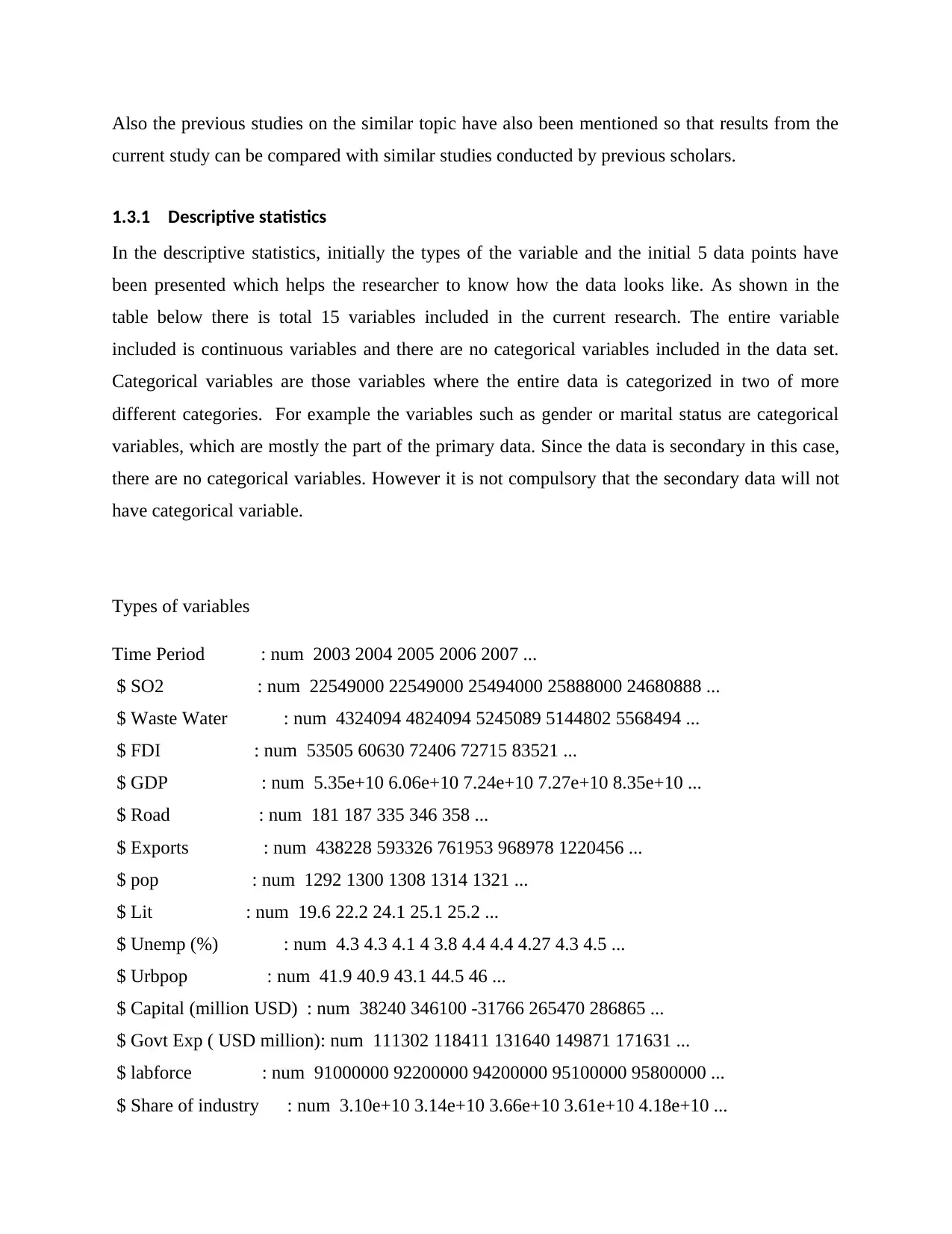
1.3.1 Descriptive statistics
In the descriptive statistics, initially the types of the variable and the initial 5 data points have
been presented which helps the researcher to know how the data looks like. As shown in the
table below there is total 15 variables included in the current research. The entire variable
included is continuous variables and there are no categorical variables included in the data set.
Categorical variables are those variables where the entire data is categorized in two of more
different categories. For example the variables such as gender or marital status are categorical
variables, which are mostly the part of the primary data. Since the data is secondary in this case,
there are no categorical variables. However it is not compulsory that the secondary data will not
have categorical variable.
Types of variables
Time Period : num 2003 2004 2005 2006 2007 ...
$ SO2 : num 22549000 22549000 25494000 25888000 24680888 ...
$ Waste Water : num 4324094 4824094 5245089 5144802 5568494 ...
$ FDI : num 53505 60630 72406 72715 83521 ...
$ GDP : num 5.35e+10 6.06e+10 7.24e+10 7.27e+10 8.35e+10 ...
$ Road : num 181 187 335 346 358 ...
$ Exports : num 438228 593326 761953 968978 1220456 ...
$ pop : num 1292 1300 1308 1314 1321 ...
$ Lit : num 19.6 22.2 24.1 25.1 25.2 ...
$ Unemp (%) : num 4.3 4.3 4.1 4 3.8 4.4 4.4 4.27 4.3 4.5 ...
$ Urbpop : num 41.9 40.9 43.1 44.5 46 ...
$ Capital (million USD) : num 38240 346100 -31766 265470 286865 ...
$ Govt Exp ( USD million): num 111302 118411 131640 149871 171631 ...
$ labforce : num 91000000 92200000 94200000 95100000 95800000 ...
$ Share of industry : num 3.10e+10 3.14e+10 3.66e+10 3.61e+10 4.18e+10 ...

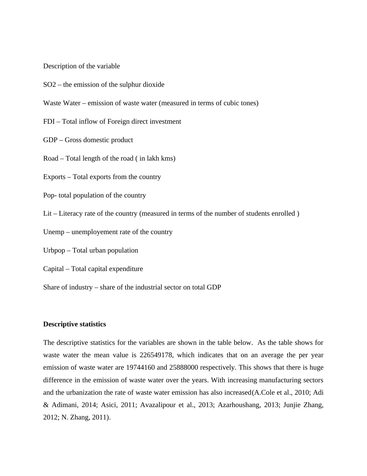
Description of the variable
SO2 – the emission of the sulphur dioxide
Waste Water – emission of waste water (measured in terms of cubic tones)
FDI – Total inflow of Foreign direct investment
GDP – Gross domestic product
Road – Total length of the road ( in lakh kms)
Exports – Total exports from the country
Pop- total population of the country
Lit – Literacy rate of the country (measured in terms of the number of students enrolled )
Unemp – unemployement rate of the country
Urbpop – Total urban population
Capital – Total capital expenditure
Share of industry – share of the industrial sector on total GDP
Descriptive statistics
The descriptive statistics for the variables are shown in the table below. As the table shows for
waste water the mean value is 226549178, which indicates that on an average the per year
emission of waste water are 19744160 and 25888000 respectively. This shows that there is huge
difference in the emission of waste water over the years. With increasing manufacturing sectors
and the urbanization the rate of waste water emission has also increased(A.Cole et al., 2010; Adi
& Adimani, 2014; Asici, 2011; Avazalipour et al., 2013; Azarhoushang, 2013; Junjie Zhang,
2012; N. Zhang, 2011).

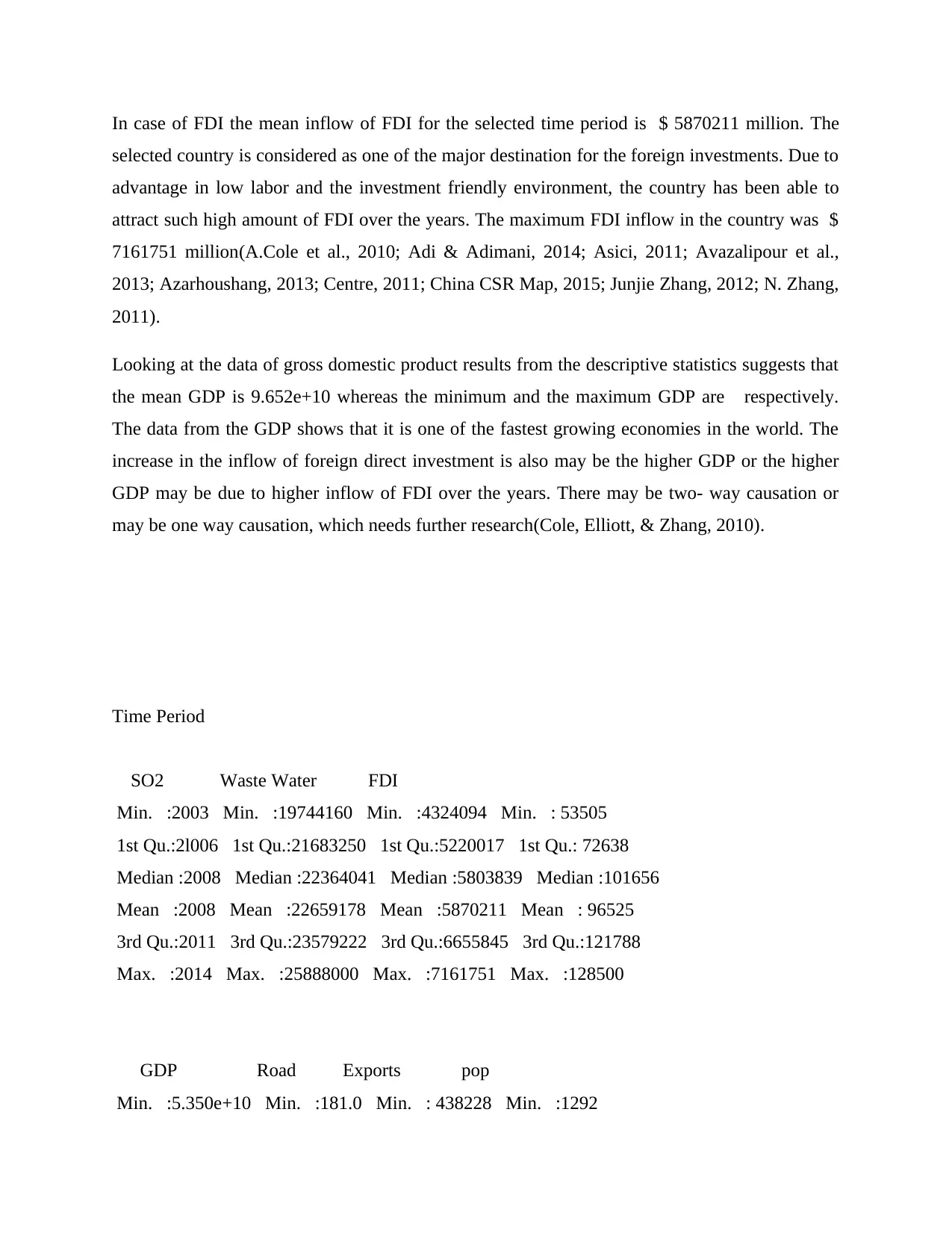
In case of FDI the mean inflow of FDI for the selected time period is $ 5870211 million. The
selected country is considered as one of the major destination for the foreign investments. Due to
advantage in low labor and the investment friendly environment, the country has been able to
attract such high amount of FDI over the years. The maximum FDI inflow in the country was $
7161751 million(A.Cole et al., 2010; Adi & Adimani, 2014; Asici, 2011; Avazalipour et al.,
2013; Azarhoushang, 2013; Centre, 2011; China CSR Map, 2015; Junjie Zhang, 2012; N. Zhang,
2011).
Looking at the data of gross domestic product results from the descriptive statistics suggests that
the mean GDP is 9.652e+10 whereas the minimum and the maximum GDP are respectively.
The data from the GDP shows that it is one of the fastest growing economies in the world. The
increase in the inflow of foreign direct investment is also may be the higher GDP or the higher
GDP may be due to higher inflow of FDI over the years. There may be two- way causation or
may be one way causation, which needs further research(Cole, Elliott, & Zhang, 2010).
Time Period
SO2 Waste Water FDI
Min. :2003 Min. :19744160 Min. :4324094 Min. : 53505
1st Qu.:2l006 1st Qu.:21683250 1st Qu.:5220017 1st Qu.: 72638
Median :2008 Median :22364041 Median :5803839 Median :101656
Mean :2008 Mean :22659178 Mean :5870211 Mean : 96525
3rd Qu.:2011 3rd Qu.:23579222 3rd Qu.:6655845 3rd Qu.:121788
Max. :2014 Max. :25888000 Max. :7161751 Max. :128500
GDP Road Exports pop
Min. :5.350e+10 Min. :181.0 Min. : 438228 Min. :1292

1st Qu.:7.264e+10 1st Qu.:342.9 1st Qu.: 917222 1st Qu.:1312
Median :1.017e+11 Median :379.6 Median :1325575 Median :1332
Mean :9.652e+10 Mean :353.1 Mean :1390949 Mean :1331
3rd Qu.:1.218e+11 3rd Qu.:403.3 3rd Qu.:1935964 3rd Qu.:1349
Max. :1.285e+11 Max. :435.6 Max. :2342293 Max. :1368
Lit Unemp (%) Urbpop Capital (million USD)
Min. :19.65 Min. :3.800 Min. :40.88 Min. :-31766
1st Qu.:24.07 1st Qu.:4.228 1st Qu.:44.12 1st Qu.: 47011
Median :24.35 Median :4.300 Median :47.78 Median : 94790
Mean :23.94 Mean :4.306 Mean :47.90 Mean :128785
3rd Qu.:24.69 3rd Qu.:4.425 3rd Qu.:51.72 3rd Qu.:215220
Max. :25.22 Max. :4.700 Max. :54.91 Max. :346100
Govt Exp ( USD million) labforce Share of industry
Min. :111302 Min. : 91000000 Min. :3.098e+10
1st Qu.:145313 1st Qu.: 94875000 1st Qu.:3.646e+10
Median :214500 Median : 97100000 Median :4.864e+10
Mean :210542 Mean : 97016667 Mean :4.887e+10
3rd Qu.:256151 3rd Qu.:100325000 3rd Qu.:6.067e+10
Max. :338551 Max. :100600000 Max. :6.586e+10
Similarly, the table shows that the average population of the country is 1131 million with
maximum population of 1368 million in the latest year and 1291 in the starting year included in
the current study. As the data suggests, the selected country has highest population in the world.
The median population is 1332 which suggest some different in the mean population and the
median population. Many scholars argue that the median is better measure of central tendency as
compared to mean. This is because mean value is affected by the extreme values which is not the
case in median values. The results from the literature review show that the average literacy rate

of the country is 23.94 which is not high as compared to other developed nations which suggests
that the selected country is still in the developing phase. Even the growth rate is one of the
highest; country is facing issues related to development(Hooda, No, Under, & Kumar, 2011;
Mukherjee, 2012). Being the higher populated country can be one of the main reasons behind
slow development in the country. Similarly the urban population is also increasing continuously.
On an average 47.90 % of the total population lives in the urban area. Due to rapid urbanization
without the proper planning the problem of environmental pollution is coming up, which is one
of the key area, this research is aimed to find(China CSR Map, 2015; Hogan Lovells, 2014; Seto,
2009).
1.3.2 Histograms
Results from histogram are shown in following section. Histograms have constructed only for
those variables which are taken as the dependent variable on the regression analysis. The
histogram of the FDI is shown in the figure below. Histograms are mainly constructed to
examine the data structure. Usually the inference analysis is conducted if the data follows normal
distribution. In case of the normal distribution most of the data around mean and there is no
significant number of outliers in the data set.

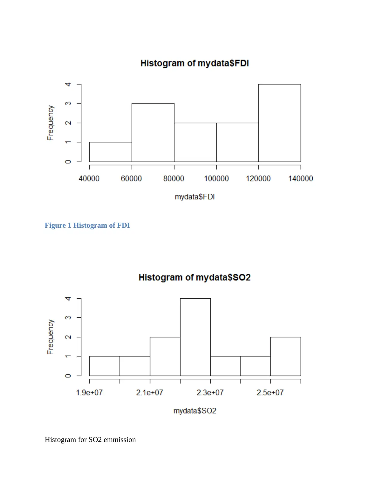
Figure 1 Histogram of FDI
Histogram for SO2 emmission

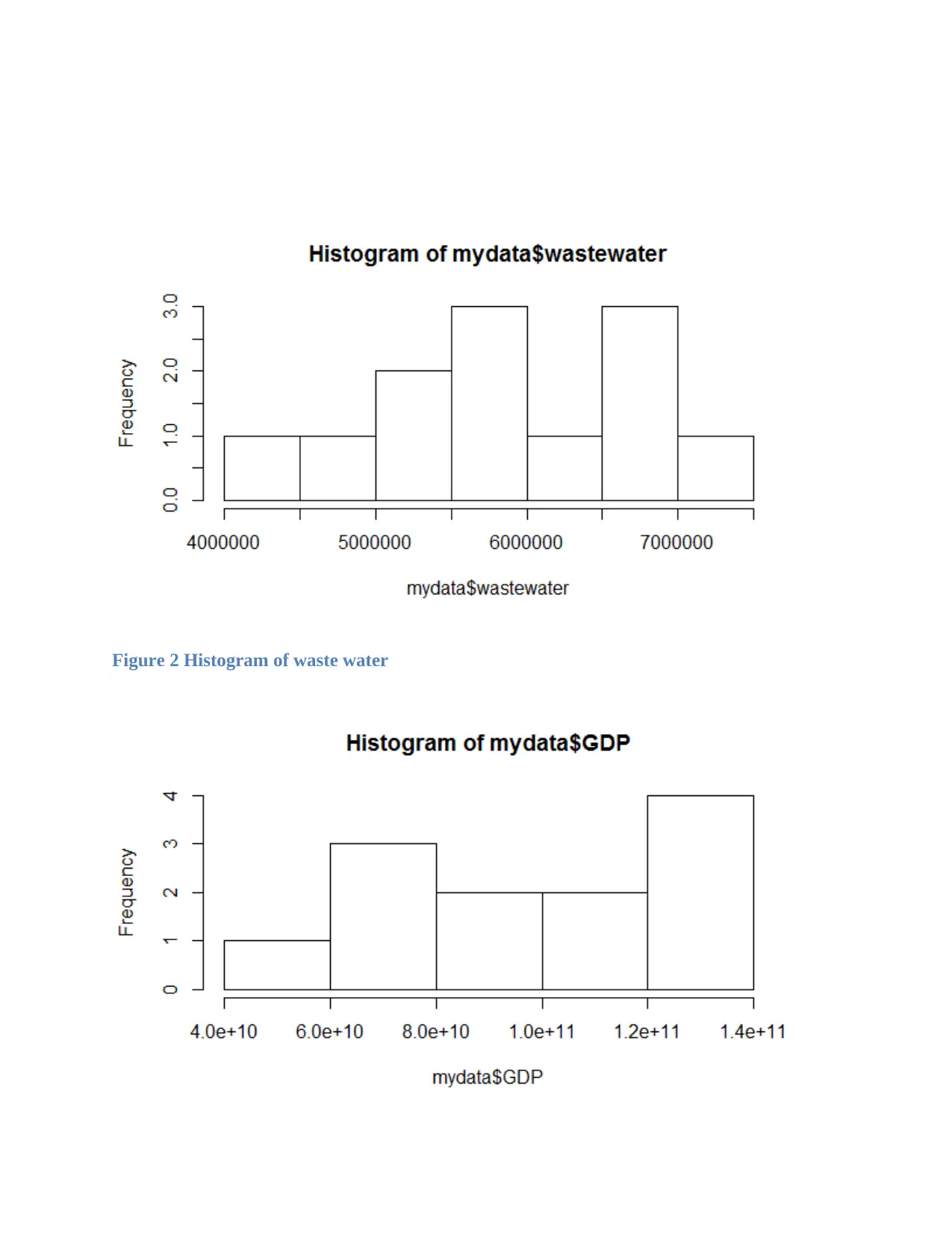
Figure 2 Histogram of waste water

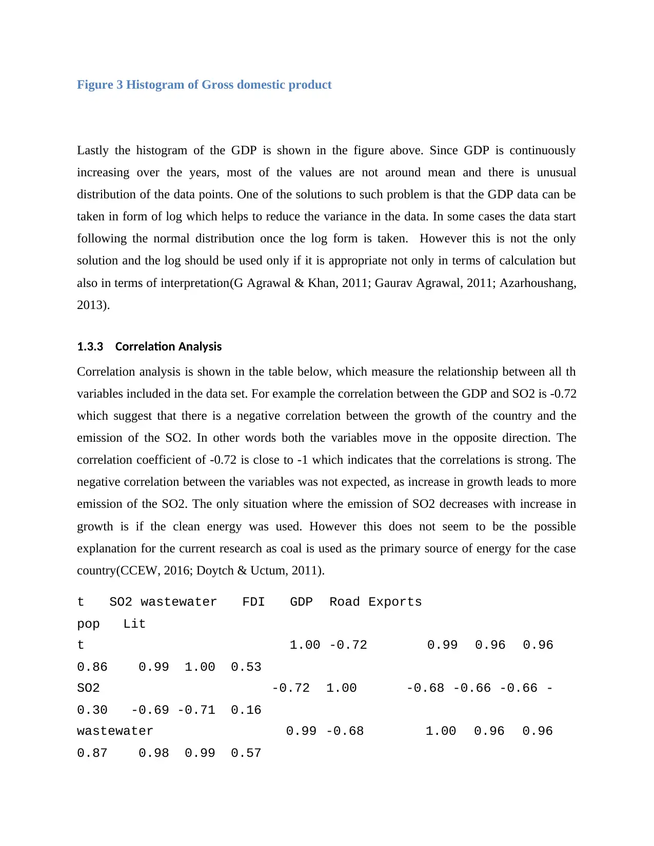
Figure 3 Histogram of Gross domestic product
Lastly the histogram of the GDP is shown in the figure above. Since GDP is continuously
increasing over the years, most of the values are not around mean and there is unusual
distribution of the data points. One of the solutions to such problem is that the GDP data can be
taken in form of log which helps to reduce the variance in the data. In some cases the data start
following the normal distribution once the log form is taken. However this is not the only
solution and the log should be used only if it is appropriate not only in terms of calculation but
also in terms of interpretation(G Agrawal & Khan, 2011; Gaurav Agrawal, 2011; Azarhoushang,
2013).
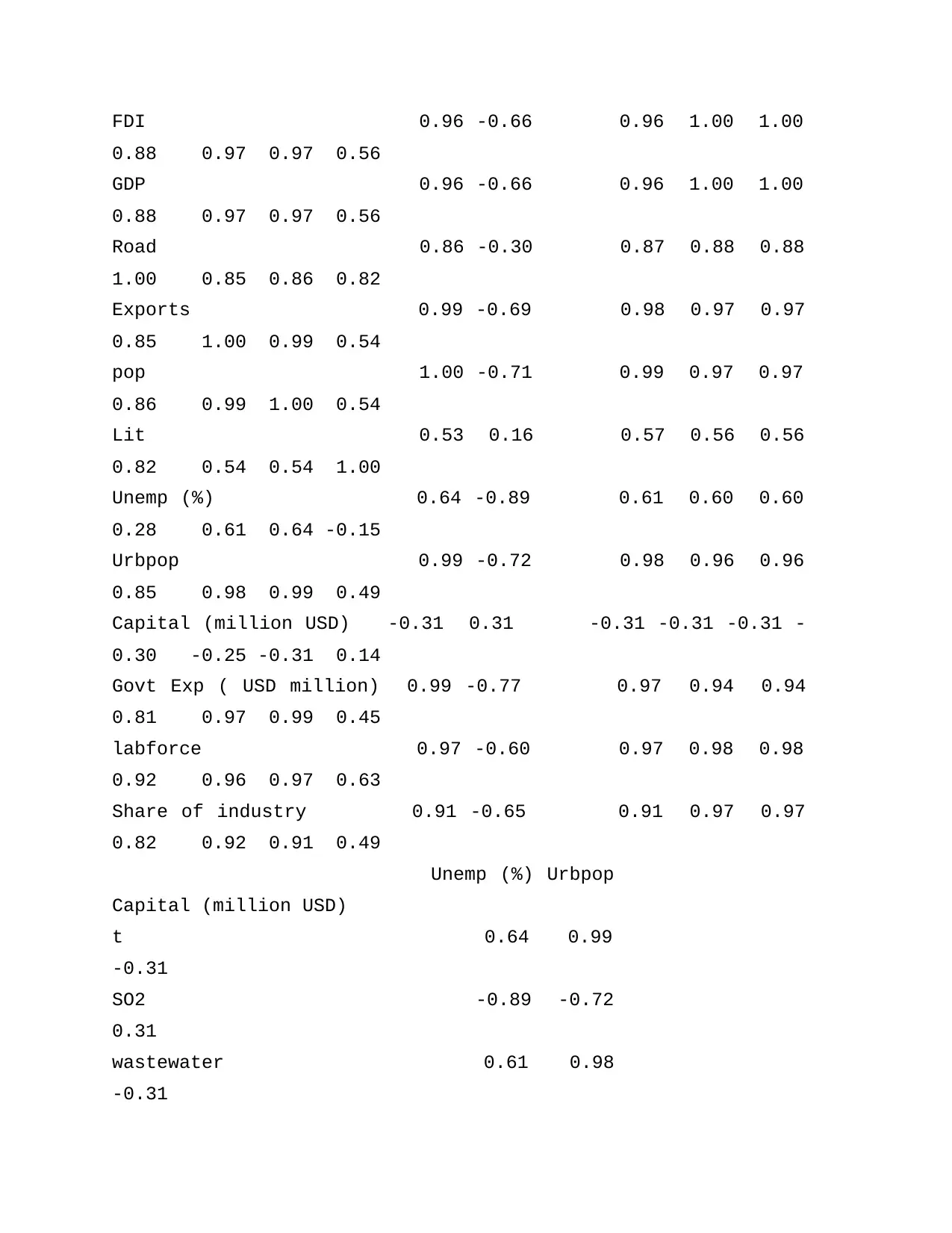
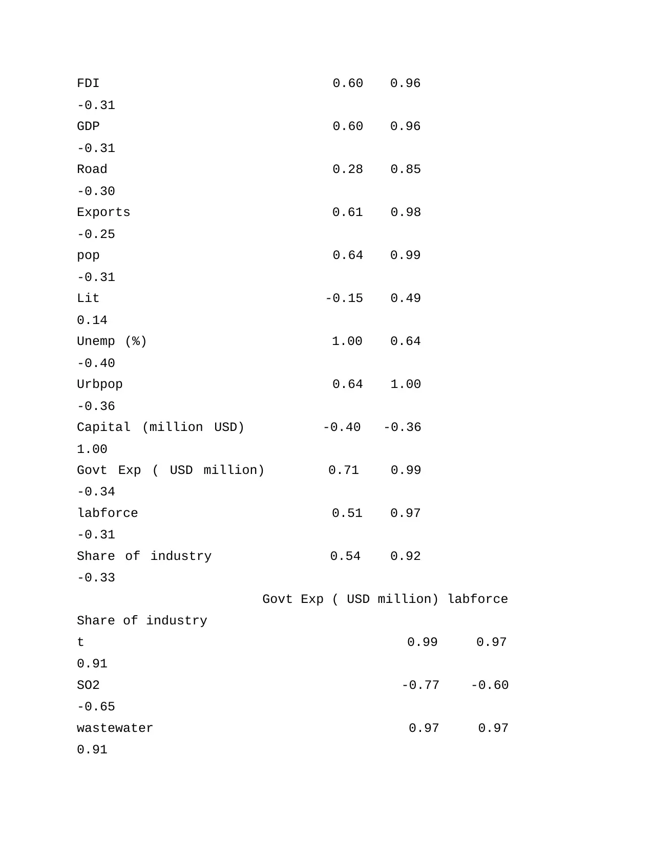
1.3.3 Correlation Analysis
Correlation analysis is shown in the table below, which measure the relationship between all th
variables included in the data set. For example the correlation between the GDP and SO2 is -0.72
which suggest that there is a negative correlation between the growth of the country and the
emission of the SO2. In other words both the variables move in the opposite direction. The
correlation coefficient of -0.72 is close to -1 which indicates that the correlations is strong. The
negative correlation between the variables was not expected, as increase in growth leads to more
emission of the SO2. The only situation where the emission of SO2 decreases with increase in
growth is if the clean energy was used. However this does not seem to be the possible
explanation for the current research as coal is used as the primary source of energy for the case
country(CCEW, 2016; Doytch & Uctum, 2011).
t SO2 wastewater FDI GDP Road Exports
pop Lit
t 1.00 -0.72 0.99 0.96 0.96
0.86 0.99 1.00 0.53
SO2 -0.72 1.00 -0.68 -0.66 -0.66 -
0.30 -0.69 -0.71 0.16
wastewater 0.99 -0.68 1.00 0.96 0.96
0.87 0.98 0.99 0.57

FDI 0.96 -0.66 0.96 1.00 1.00
0.88 0.97 0.97 0.56
GDP 0.96 -0.66 0.96 1.00 1.00
0.88 0.97 0.97 0.56
Road 0.86 -0.30 0.87 0.88 0.88
1.00 0.85 0.86 0.82
Exports 0.99 -0.69 0.98 0.97 0.97
0.85 1.00 0.99 0.54
pop 1.00 -0.71 0.99 0.97 0.97
0.86 0.99 1.00 0.54
Lit 0.53 0.16 0.57 0.56 0.56
0.82 0.54 0.54 1.00
Unemp (%) 0.64 -0.89 0.61 0.60 0.60
0.28 0.61 0.64 -0.15
Urbpop 0.99 -0.72 0.98 0.96 0.96
0.85 0.98 0.99 0.49
Capital (million USD) -0.31 0.31 -0.31 -0.31 -0.31 -
0.30 -0.25 -0.31 0.14
Govt Exp ( USD million) 0.99 -0.77 0.97 0.94 0.94
0.81 0.97 0.99 0.45
labforce 0.97 -0.60 0.97 0.98 0.98
0.92 0.96 0.97 0.63
Share of industry 0.91 -0.65 0.91 0.97 0.97
0.82 0.92 0.91 0.49
Unemp (%) Urbpop
Capital (million USD)
t 0.64 0.99
-0.31
SO2 -0.89 -0.72
0.31
wastewater 0.61 0.98
-0.31

FDI 0.60 0.96
-0.31
GDP 0.60 0.96
-0.31
Road 0.28 0.85
-0.30
Exports 0.61 0.98
-0.25
pop 0.64 0.99
-0.31
Lit -0.15 0.49
0.14
Unemp (%) 1.00 0.64
-0.40
Urbpop 0.64 1.00
-0.36
Capital (million USD) -0.40 -0.36
1.00
Govt Exp ( USD million) 0.71 0.99
-0.34
labforce 0.51 0.97
-0.31
Share of industry 0.54 0.92
-0.33
Govt Exp ( USD million) labforce
Share of industry
t 0.99 0.97
0.91
SO2 -0.77 -0.60
-0.65
wastewater 0.97 0.97
0.91