Macroeconomics

This document provides study material and solved assignments on various topics in macroeconomics. It covers concepts such as GDP, consumption, investment, government expenditure, and more. The data is collected from the Australian Bureau of Statistics. The document also discusses the impact of monetary and fiscal policies, as well as the potential effects of the US-China trade war on the Australian economy.

Running head: MACROECONOMICS
Macroeconomics
Name of the Student:
Name of the University:
Author Note:

1MACROECONOMICS
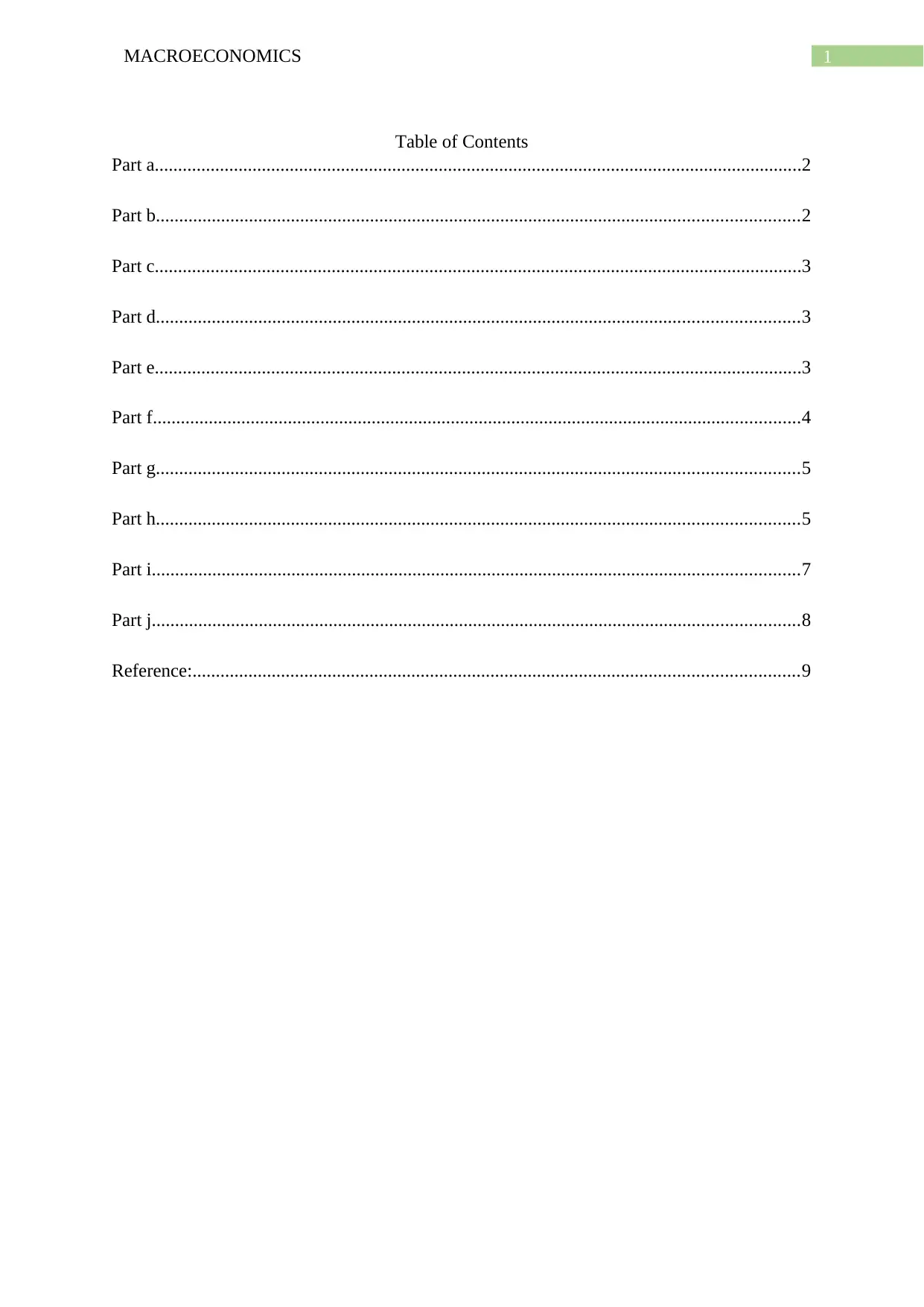
Table of Contents
Part a...........................................................................................................................................2
Part b..........................................................................................................................................2
Part c...........................................................................................................................................3
Part d..........................................................................................................................................3
Part e...........................................................................................................................................3
Part f...........................................................................................................................................4
Part g..........................................................................................................................................5
Part h..........................................................................................................................................5
Part i...........................................................................................................................................7
Part j...........................................................................................................................................8
Reference:..................................................................................................................................9

2MACROECONOMICS
Part a
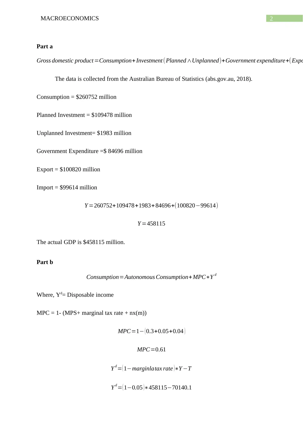
Gross domestic product =Consumption+ Investment (Planned ∧Unplanned)+Government expenditure+( Expo
The data is collected from the Australian Bureau of Statistics (abs.gov.au, 2018).
Consumption = $260752 million
Planned Investment = $109478 million
Unplanned Investment= $1983 million
Government Expenditure =$ 84696 million
Export = $100820 million
Import = $99614 million
Y =260752+109478+1983+ 84696+(100820−99614)
Y =458115
The actual GDP is $458115 million.
Part b
Consumption=Autonomous Consumption+ MPC∗Y d
Where, Yd= Disposable income
MPC = 1- (MPS+ marginal tax rate + nx(m))
MPC=1− ( 0.3+0.05+0.04 )
MPC=0.61
Y d = ( 1−marginlatax rate )∗Y −T
Y d = ( 1−0.05 )∗458115−70140.1

3MACROECONOMICS
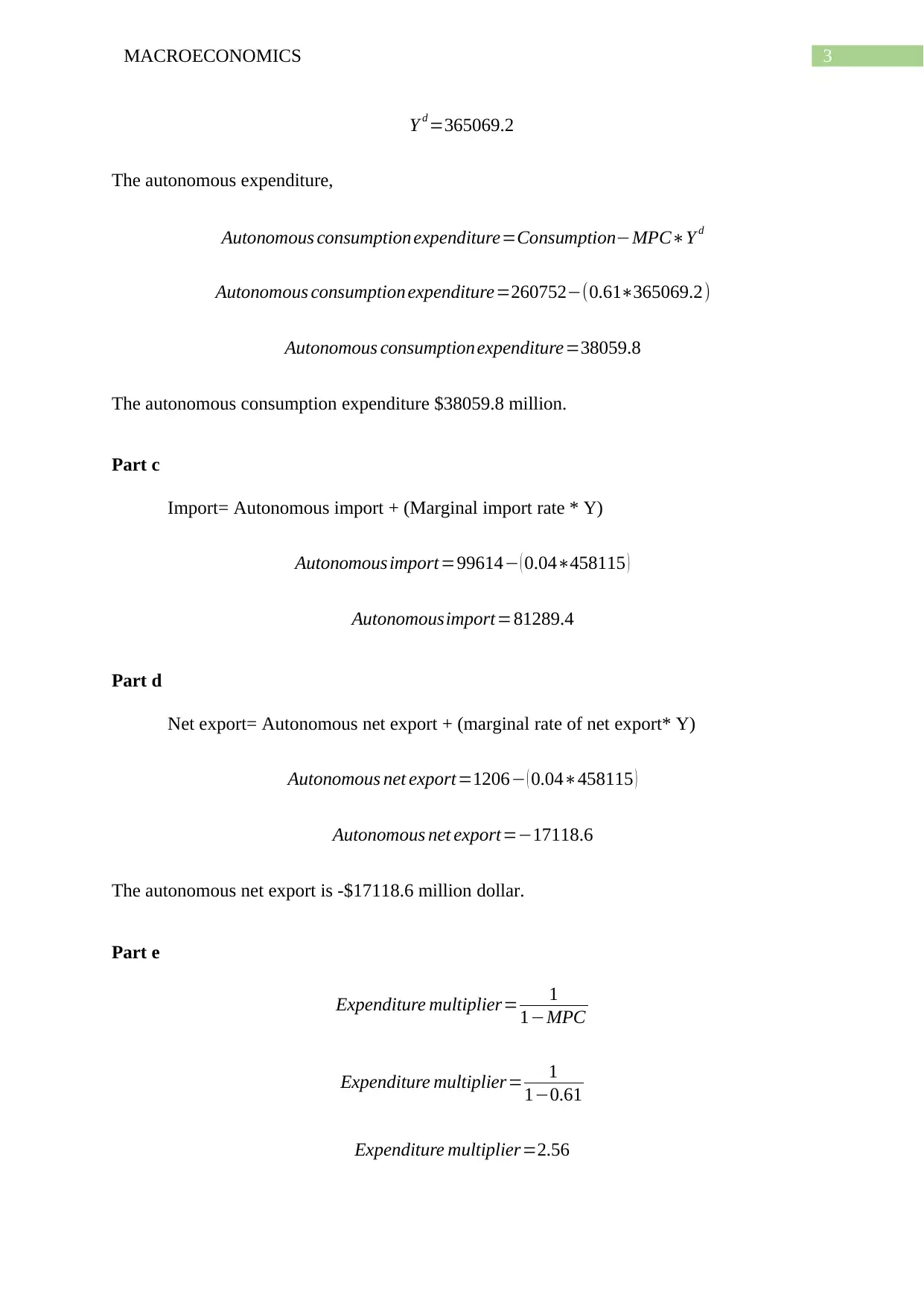
Y d =365069.2
The autonomous expenditure,
Autonomous consumption expenditure=Consumption−MPC∗Y d
Autonomous consumption expenditure=260752−(0.61∗365069.2)
Autonomous consumptionexpenditure=38059.8
The autonomous consumption expenditure $38059.8 million.
Part c
Import= Autonomous import + (Marginal import rate * Y)
Autonomousimport=99614− ( 0.04∗458115 )
Autonomousimport=81289.4
Part d
Net export= Autonomous net export + (marginal rate of net export* Y)
Autonomous net export=1206− ( 0.04∗458115 )
Autonomous net export=−17118.6
The autonomous net export is -$17118.6 million dollar.
Part e
Expenditure multiplier= 1
1−MPC
Expenditure multiplier= 1
1−0.61
Expenditure multiplier=2.56

4MACROECONOMICS
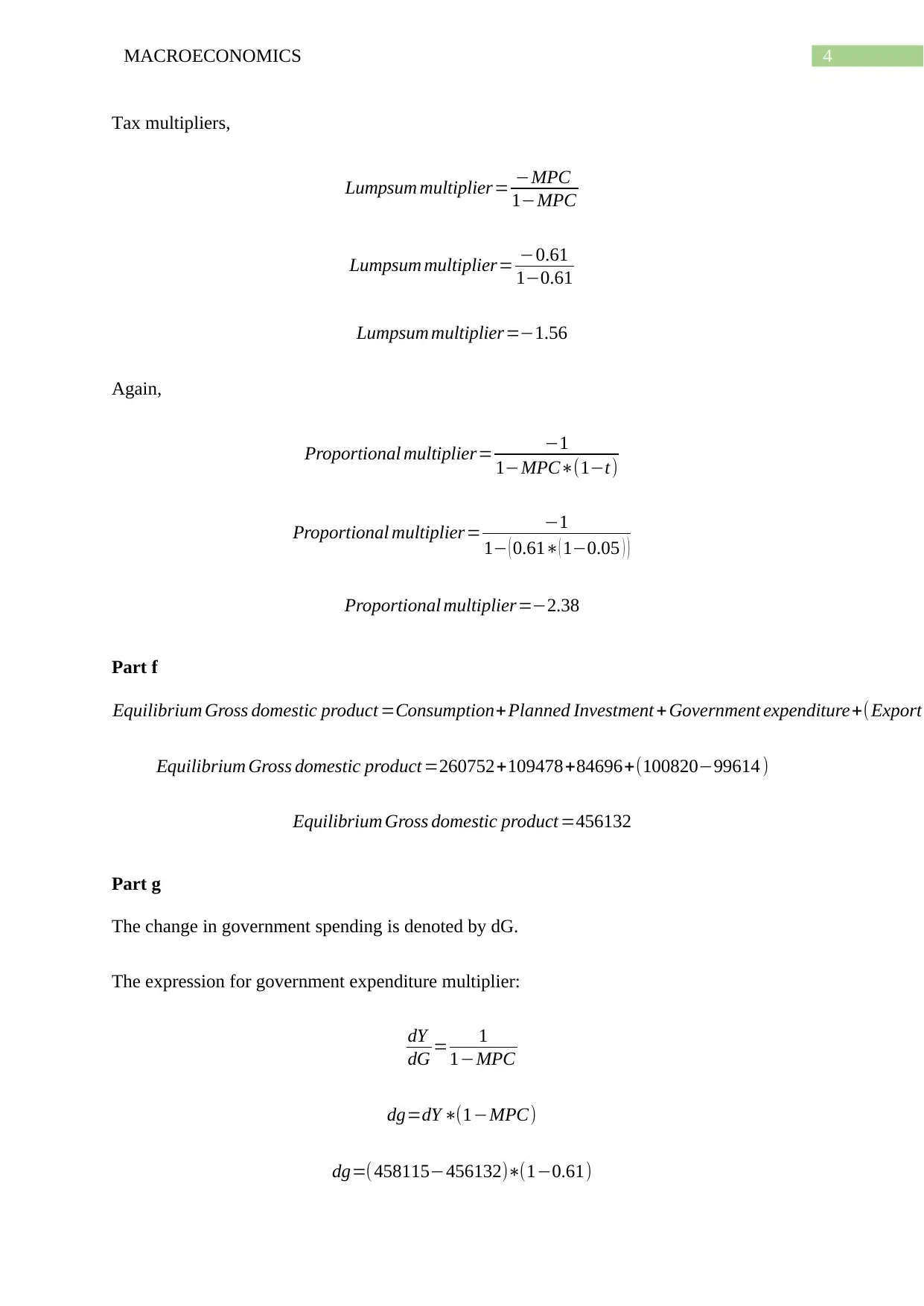
Tax multipliers,
Lumpsum multiplier= −MPC
1−MPC
Lumpsum multiplier= −0.61
1−0.61
Lumpsum multiplier=−1.56
Again,
Proportional multiplier= −1
1−MPC∗(1−t)
Proportional multiplier= −1
1− ( 0.61∗( 1−0.05 ) )
Proportional multiplier=−2.38
Part f
Equilibrium Gross domestic product =Consumption+ Planned Investment + Government expenditure+(Export
Equilibrium Gross domestic product =260752+109478+84696+(100820−99614 )
Equilibrium Gross domestic product =456132
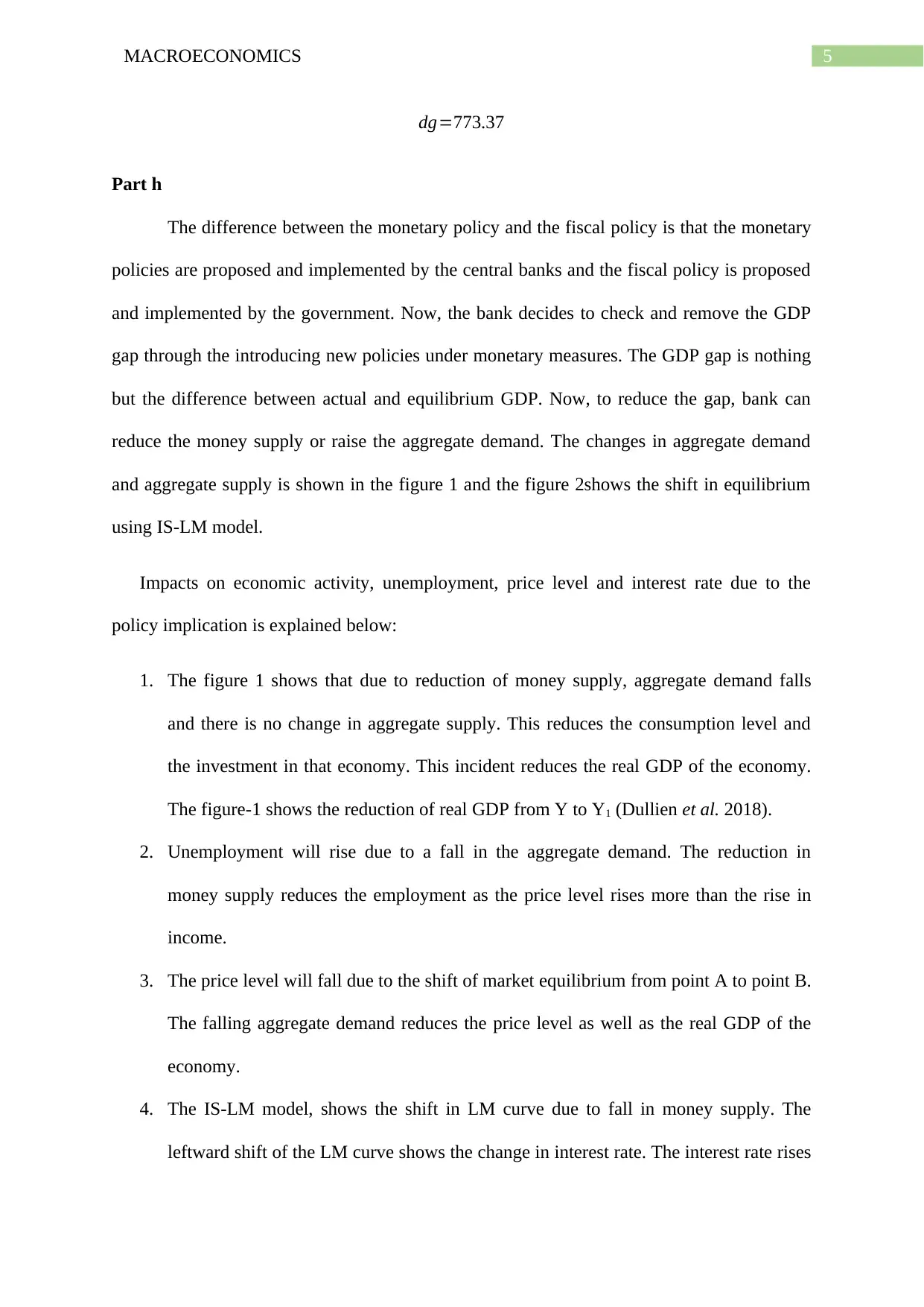
Part g
The change in government spending is denoted by dG.
The expression for government expenditure multiplier:
dY
dG = 1
1−MPC
dg=dY ∗(1−MPC)
dg=(458115−456132)∗(1−0.61)

5MACROECONOMICS
dg=773.37
Part h
The difference between the monetary policy and the fiscal policy is that the monetary
policies are proposed and implemented by the central banks and the fiscal policy is proposed
and implemented by the government. Now, the bank decides to check and remove the GDP
gap through the introducing new policies under monetary measures. The GDP gap is nothing
but the difference between actual and equilibrium GDP. Now, to reduce the gap, bank can
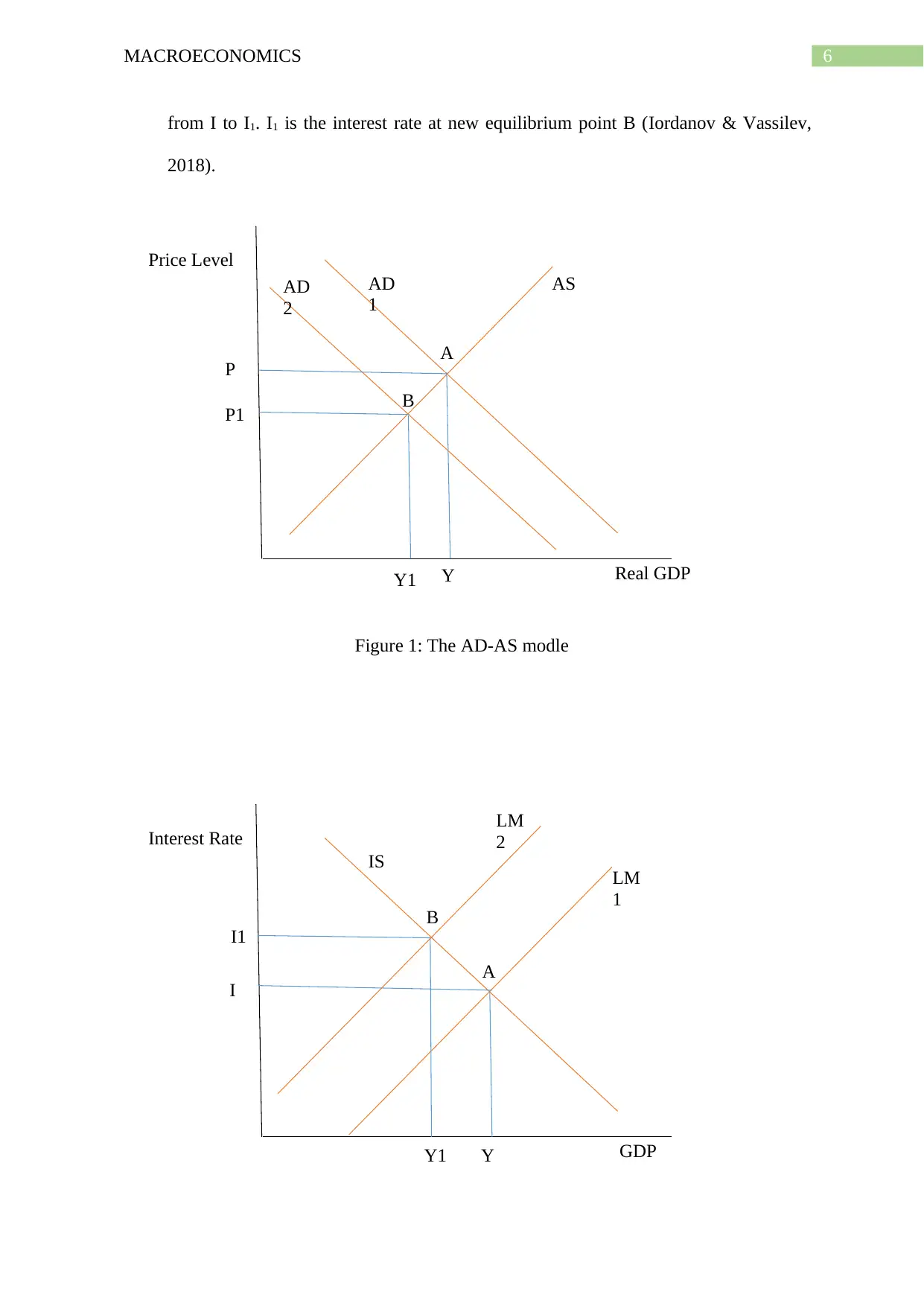
reduce the money supply or raise the aggregate demand. The changes in aggregate demand
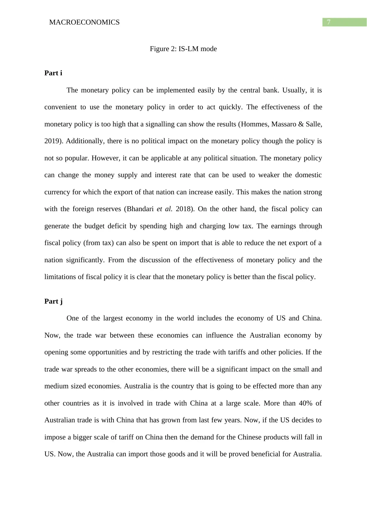
and aggregate supply is shown in the figure 1 and the figure 2shows the shift in equilibrium
using IS-LM model.
Impacts on economic activity, unemployment, price level and interest rate due to the
policy implication is explained below:
1. The figure 1 shows that due to reduction of money supply, aggregate demand falls
and there is no change in aggregate supply. This reduces the consumption level and
the investment in that economy. This incident reduces the real GDP of the economy.
The figure-1 shows the reduction of real GDP from Y to Y1 (Dullien et al. 2018).
2. Unemployment will rise due to a fall in the aggregate demand. The reduction in
money supply reduces the employment as the price level rises more than the rise in
income.
3. The price level will fall due to the shift of market equilibrium from point A to point B.
The falling aggregate demand reduces the price level as well as the real GDP of the
economy.
4. The IS-LM model, shows the shift in LM curve due to fall in money supply. The
leftward shift of the LM curve shows the change in interest rate. The interest rate rises

6MACROECONOMICS
Price Level
Real GDP
AS
Y1 Y
P1
P
AD
2
AD
1
A
B
Interest Rate
GDP
LM
1
Y1 Y
I1
I
LM
2
IS
B
A
from I to I1. I1 is the interest rate at new equilibrium point B (Iordanov & Vassilev,
2018).
Figure 1: The AD-AS modle

7MACROECONOMICS
Figure 2: IS-LM mode
Part i
The monetary policy can be implemented easily by the central bank. Usually, it is
convenient to use the monetary policy in order to act quickly. The effectiveness of the
monetary policy is too high that a signalling can show the results (Hommes, Massaro & Salle,
2019). Additionally, there is no political impact on the monetary policy though the policy is
not so popular. However, it can be applicable at any political situation. The monetary policy
can change the money supply and interest rate that can be used to weaker the domestic
currency for which the export of that nation can increase easily. This makes the nation strong
with the foreign reserves (Bhandari et al. 2018). On the other hand, the fiscal policy can
generate the budget deficit by spending high and charging low tax. The earnings through
fiscal policy (from tax) can also be spent on import that is able to reduce the net export of a
nation significantly. From the discussion of the effectiveness of monetary policy and the
limitations of fiscal policy it is clear that the monetary policy is better than the fiscal policy.
Part j
One of the largest economy in the world includes the economy of US and China.
Now, the trade war between these economies can influence the Australian economy by
opening some opportunities and by restricting the trade with tariffs and other policies. If the
trade war spreads to the other economies, there will be a significant impact on the small and
medium sized economies. Australia is the country that is going to be effected more than any
other countries as it is involved in trade with China at a large scale. More than 40% of
Australian trade is with China that has grown from last few years. Now, if the US decides to
impose a bigger scale of tariff on China then the demand for the Chinese products will fall in
US. Now, the Australia can import those goods and it will be proved beneficial for Australia.

8MACROECONOMICS
However, there are few trade settlements between US and China that can worsen the trade
situation of Australia and China. The trade war can force the Chinese economy to contract
that will reduce the export of China and subsequently there will be a reduction in the import
demand (Herrero, Xu, & Gary, 2018). This will directly affect the Australian export to China
which can reduce the employment in Australia.

9MACROECONOMICS
Reference:
abs.gov.au 2018. 5206.0 - Australian National Accounts: National Income, Expenditure and
Product, Dec 2018. [online] Abs.gov.au. Available at:
https://www.abs.gov.au/AUSSTATS/abs@.nsf/DetailsPage/5206.0Dec%202018?
OpenDocument [Accessed 12 May 2019].
Bhandari, A., Evans, D., Golosov, M., & Sargent, T. J. (2018). Inequality, Business Cycles,
and Monetary-Fiscal Policy (No. w24710). National Bureau of Economic Research.
Dullien, S., Goodwin, N., Harris, J. M., Nelson, J. A., Roach, B., & Torras, M.
(2018). Macroeconomics in Context. Routledge.
Herrero, A. G., Xu, J., & Gary, N. G. (2018). IS THE MARKET OVERREACTING TO
THE US-CHINA TRADE WAR? YES IF ONLY FOCUSING ON TRADE MEASURES.
Hommes, C., Massaro, D., & Salle, I. (2019). Monetary and Fiscal Policy Design at the Zero
Lower Bound: Evidence from the Lab. Economic Inquiry, 57(2), 1120-1140.
Iordanov, I., & Vassilev, A. (2018, June). A Computational Approach to Teaching the IS-LM
Model. In 2018 International Conference on High Technology for Sustainable Development
(HiTech) (pp. 1-4). IEEE.