University Macroeconomics Assignment: Problems and Solutions

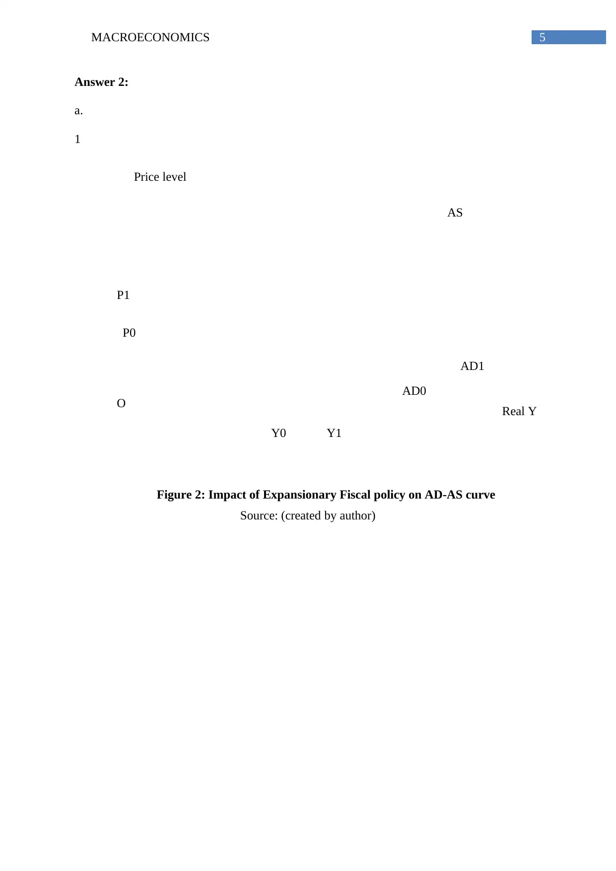
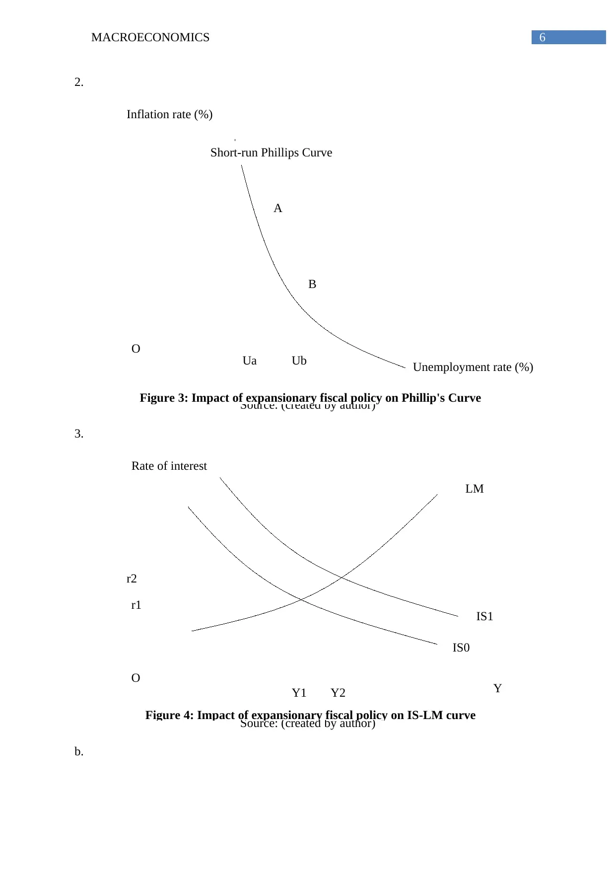
This macroeconomics assignment solution analyzes an economic model with given parameters for autonomous consumption, marginal propensity to consume, taxation, investment, government spending, and net exports. The solution calculates the equilibrium income, multiplier value, and tota...Read More

Running head: MACROECONOMICS
Macroeconomics
Name of the Student
Name of the University
Author Note

1MACROECONOMICS
Table of Contents
Answer 1:...................................................................................................................................2
Answer 2:...................................................................................................................................5
References:.................................................................................................................................8

2MACROECONOMICS
Answer 1:
Autonomous consumption (C) = 660
The marginal propensity to consume (mpc) = 0.8
Autonomous taxation (T) = 200
Planned investment (I) = 500
Government spending (G) = 500
Autonomous net exports (X-M) = 300
a.
Equilibrium value of income (Y) = C + c.(Y- T) + I+ G + (X-M)
Y =660+0.8(Y −200)+500+ 500+30 0
Y =660+0.8 Y – 160+1300
Y – 0.8 Y =1800
0.2 Y =1800
Y =9000
b.
The marginal propensity to save (MPS) = (1-0.8) = 0.2
The income tax rate = 0.2
nx or propensity to import= 0.04
Value of Multiplier = 1 / (propensity to save + the income tax rate + propensity to import)
Value of Multiplier = 1/ (0.2 + 0.2 + 0.04)
Value of Multiplier = 1/ 0.44
Value of Multiplier= 2.27
c.
Total consumption=C+mpc (Y −T )
Total consumption=660+0.8(9000 – 200)

3MACROECONOMICS
National Income
Consumption expenditure
660
O
Negative saving
Saving
Y= C+S
Total consumption=660+0.8∗8800
Total consumption=660+7040
Total consumption=7700
d.
Source: (as per author creation)
e.
National Income (Y) = Consumption (C) + Saving (S)
S = Y – C
S = 9000 – 7700
S= 1300
Hence, the value of autonomous saving is 1300
Marginal propensity to save is 1- mpc = 1 – 0.8= 0.2
Therefore, saving function is:
Figure 1: Figure 1: Consumption and saving function

4MACROECONOMICS
1300 = S + 0.2 Y
1300 = S + 0.2 * 9000
1300= S +1800
S= -500
Thus, saving function is -500+ 0.2 Y
f.
Equation of injections = I+G+X
Equations of leakages= S+T+M
Total expenditure (E) = C + I+G+ NX
E = 7700 + 500 + 500 + 300
E = 9000
Total Income (Y) = C+S+T
Y = 7700 + 1300 + 200
Y = 9200
In equilibrium, E = Y
However, in this situation, Y is greater than E and consequently leakages are not equal with
injections.
g.
According to the formula of government multiplier:
Change in income = 1/ (1 – MPC) * change in government expenditure
Government expenditure decreases by 150
Change in income = 1/ (1 – 0.8) * 150
Change in income = 5 * 150
Change in income = 750
Hence, the economy will fall by 750

5MACROECONOMICS
AS
AD0
AD1
Price level
O Real Y
P0
P1
Y0 Y1
Answer 2:
a.
1
Source: (created by author)
Figure 2: Impact of Expansionary Fiscal policy on AD-AS curve

6MACROECONOMICS
A
B
O
Inflation rate (%)
Unemployment rate (%)
Short-run Phillips Curve
UbUa
Rate of interest
O Y
LM
IS0
IS1
Y1 Y2
r1
r2
2.
Source: (created by author)
3.
Source: (created by author)
b.
Figure 3: Impact of expansionary fiscal policy on Phillip's Curve
Figure 4: Impact of expansionary fiscal policy on IS-LM curve

7MACROECONOMICS
1. Through the expansionary fiscal policy, government can increase its expenditure or
decrease taxes and this in turn can increase the aggregate demand of the economy (Drumond
and De Jesus 2016). As a result, total aggregate demand curve sifts upward.
2. Total price level will increase from P0 to P1.
3. Inflation rate will increase from B to A.
4. Interest rate will increase from r1 to r2.
5. Unemployment rate will decrease from Ub to Ua.
c.
The government takes expansionary fiscal policy to increase demand. This in turn
helps an economy to recover from recessionary period. However, expansionary fiscal policy
leads the government to experience debt due to excess government expenditure. Hence, this
increases deficit level (Johnson 2017). Expansionary fiscal policy is more effective than
monetary policy. It increases aggregate demand of the economy and directly influences
economy. On the contrary, monetary policy cannot influence economic condition directly.

8MACROECONOMICS
References:
Drumond, C.E. and De Jesus, C.S., 2016. Monetary and fiscal policy interactions in a post
Keynesian open-economy model. Journal of Post Keynesian Economics, 39(2), pp.172-186.
Johnson, H.G., 2017. Macroeconomics and monetary theory. Routledge.