Macroeconomics Assessment | Questions

Running head: MACROECONOMICS
Macroeconomics
Name of the Student
Name of the University
Course ID

1MACROECONOMICS
Table of Contents
Question 1....................................................................................................................................................................................................2
Question 2....................................................................................................................................................................................................5
Question 3..................................................................................................................................................................................................10
References..................................................................................................................................................................................................13

2MACROECONOMICS
Question 1
a)
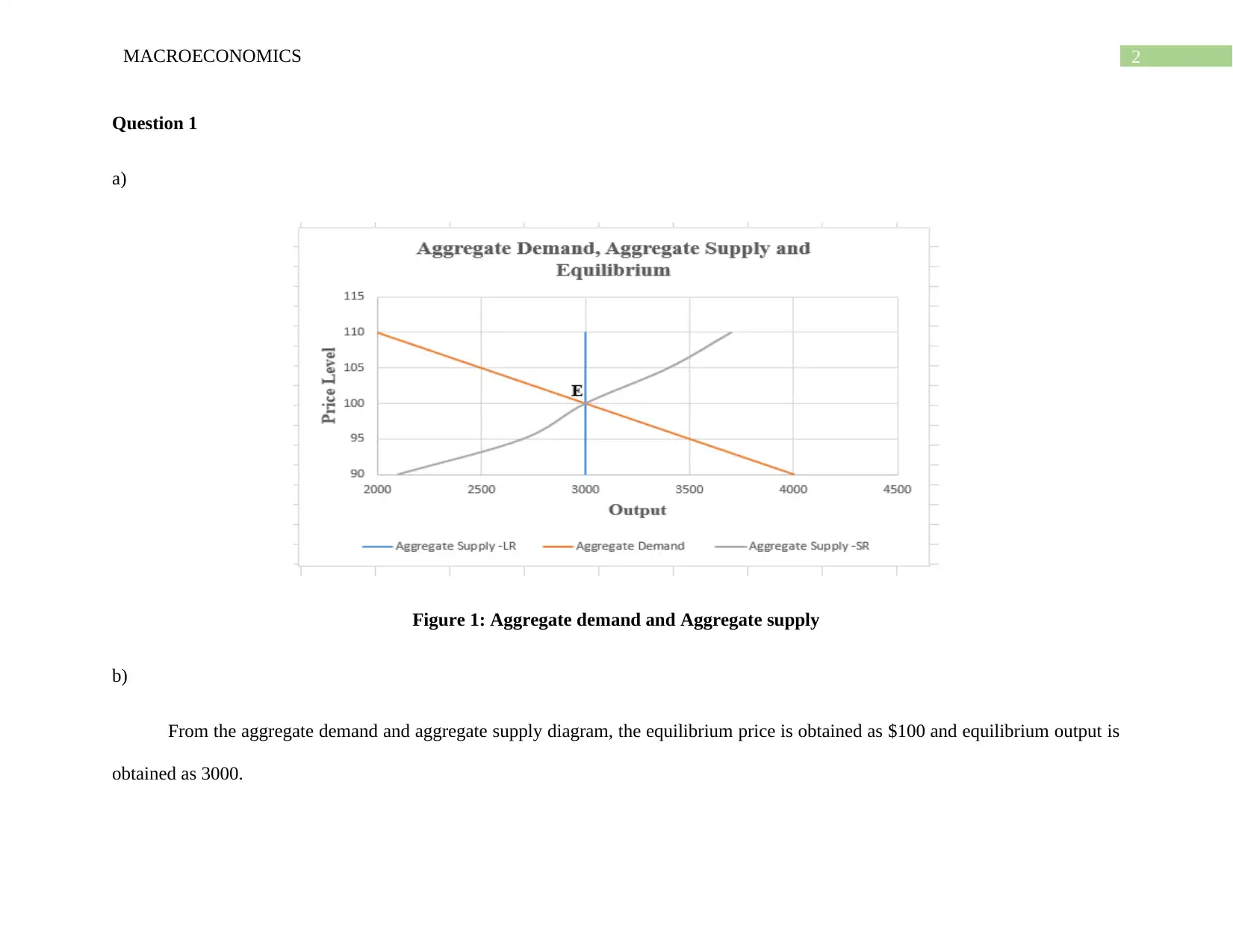
Figure 1: Aggregate demand and Aggregate supply
b)
From the aggregate demand and aggregate supply diagram, the equilibrium price is obtained as $100 and equilibrium output is
obtained as 3000.

3MACROECONOMICS
c)
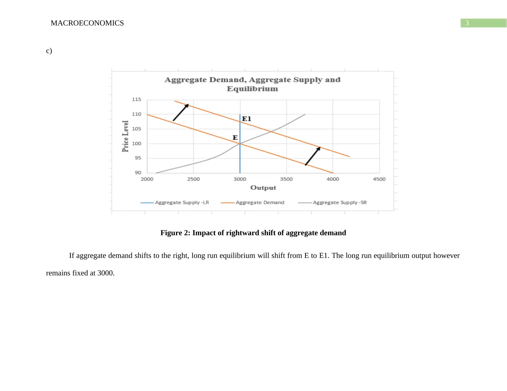
Figure 2: Impact of rightward shift of aggregate demand
If aggregate demand shifts to the right, long run equilibrium will shift from E to E1. The long run equilibrium output however
remains fixed at 3000.

4MACROECONOMICS
d)
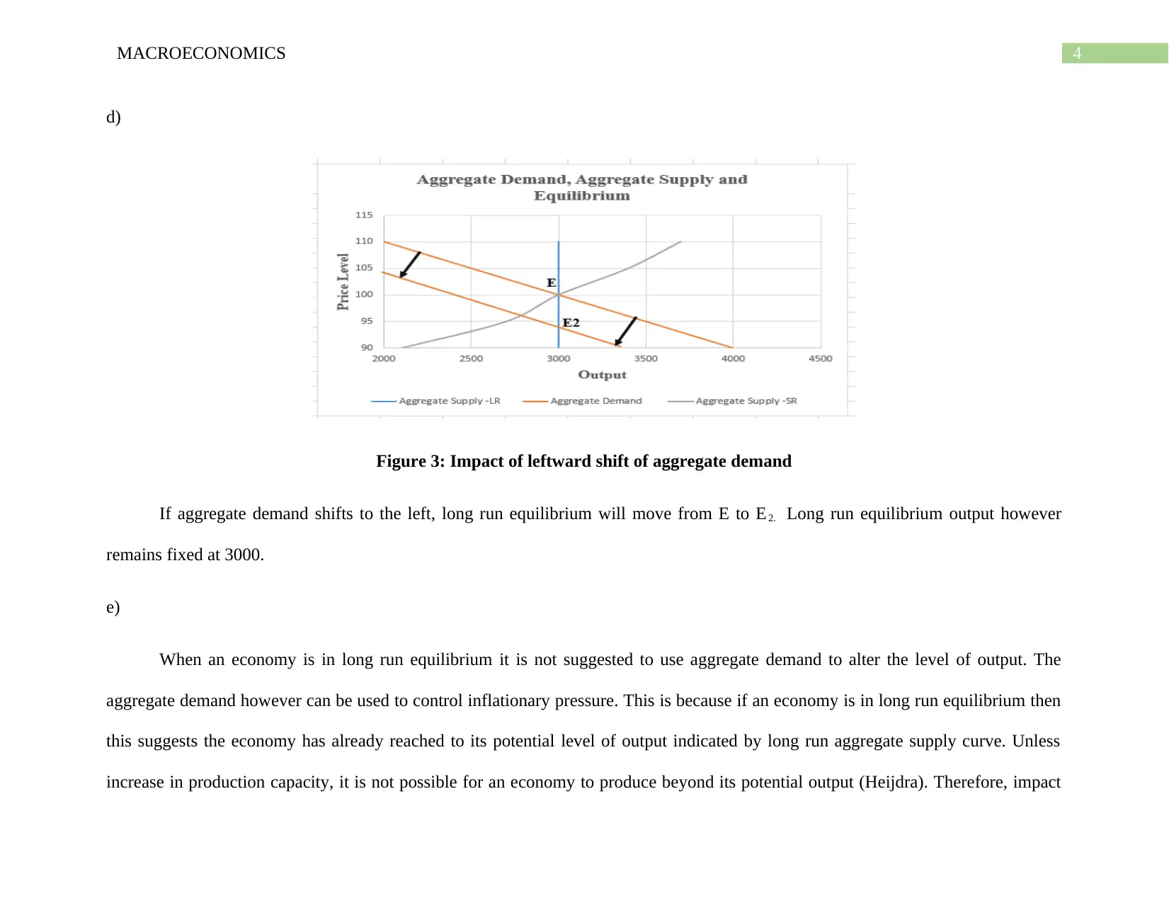
Figure 3: Impact of leftward shift of aggregate demand
If aggregate demand shifts to the left, long run equilibrium will move from E to E2. Long run equilibrium output however
remains fixed at 3000.
e)
When an economy is in long run equilibrium it is not suggested to use aggregate demand to alter the level of output. The
aggregate demand however can be used to control inflationary pressure. This is because if an economy is in long run equilibrium then
this suggests the economy has already reached to its potential level of output indicated by long run aggregate supply curve. Unless
increase in production capacity, it is not possible for an economy to produce beyond its potential output (Heijdra). Therefore, impact

5MACROECONOMICS
of any alteration of aggregate demand is limited to price level only. For controlling inflationary pressures, contractionary policies can
be taken that shifts the aggregate demand curve to the left. Decline in aggregate demand creates a downward pressure on price level
and control inflationary pressure.
Question 2
a)
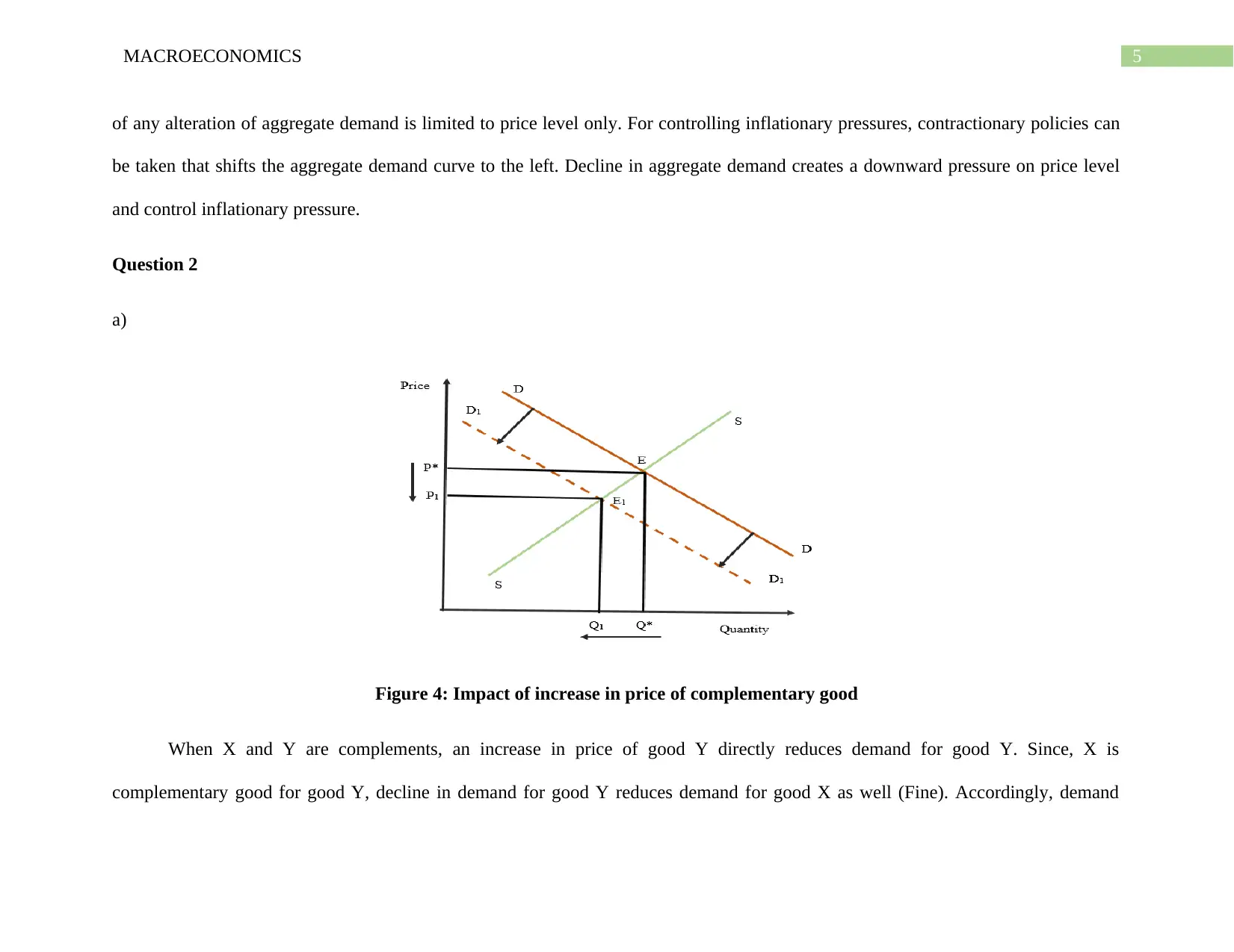
Figure 4: Impact of increase in price of complementary good
When X and Y are complements, an increase in price of good Y directly reduces demand for good Y. Since, X is
complementary good for good Y, decline in demand for good Y reduces demand for good X as well (Fine). Accordingly, demand

6MACROECONOMICS
curve for good X moves left to D1D1 from its initial position at DD. Equilibrium shifts from E to E1. Equilibrium price declines from
P* to P1 and equilibrium quantity falls from Q* to Q1.
b)
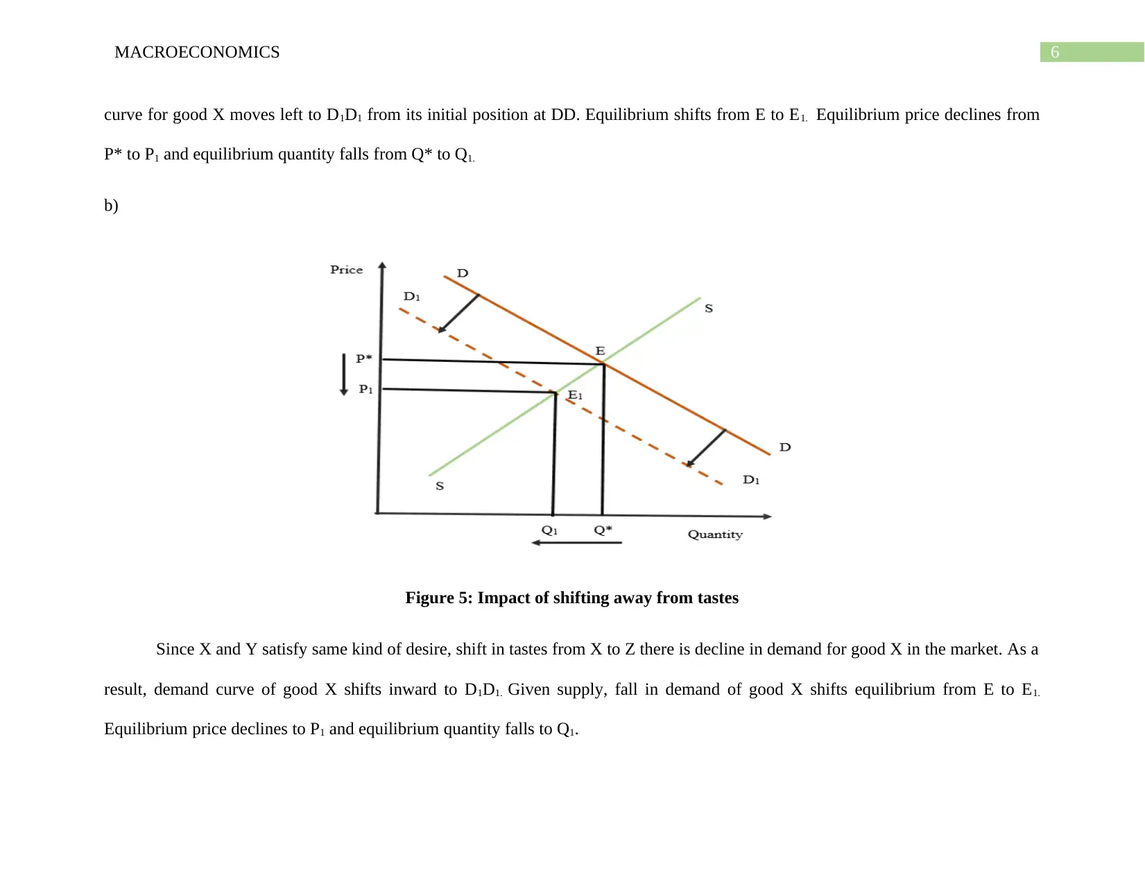
Figure 5: Impact of shifting away from tastes
Since X and Y satisfy same kind of desire, shift in tastes from X to Z there is decline in demand for good X in the market. As a
result, demand curve of good X shifts inward to D1D1. Given supply, fall in demand of good X shifts equilibrium from E to E1.
Equilibrium price declines to P1 and equilibrium quantity falls to Q1.

7MACROECONOMICS
c)
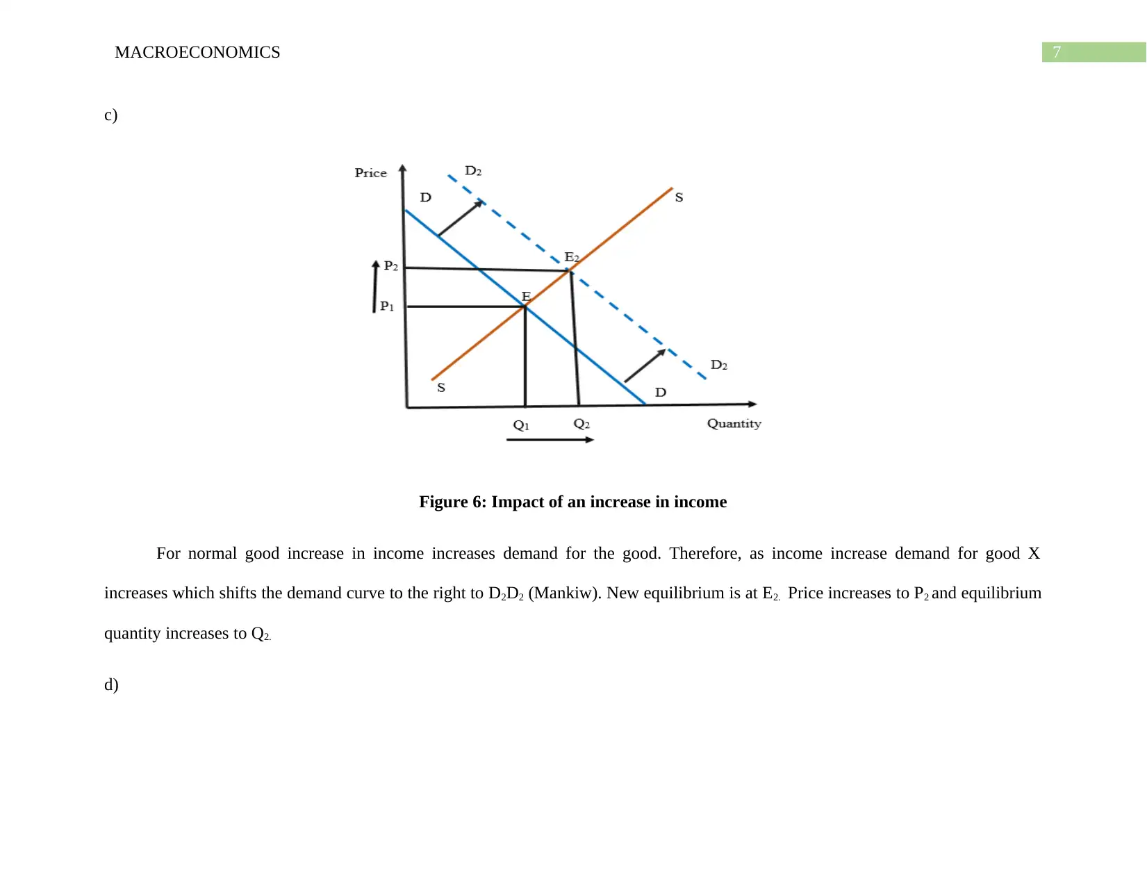
Figure 6: Impact of an increase in income
For normal good increase in income increases demand for the good. Therefore, as income increase demand for good X
increases which shifts the demand curve to the right to D2D2 (Mankiw). New equilibrium is at E2. Price increases to P2 and equilibrium
quantity increases to Q2.
d)

8MACROECONOMICS
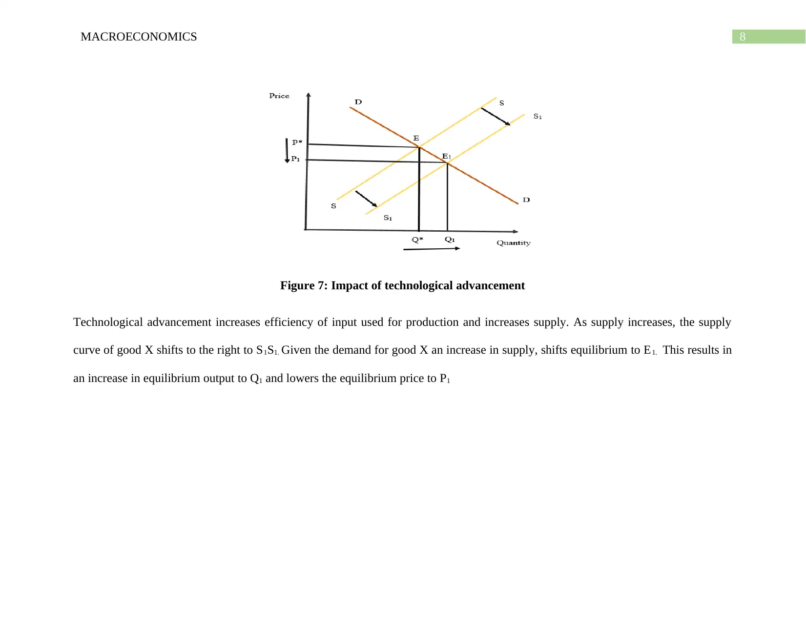
Figure 7: Impact of technological advancement
Technological advancement increases efficiency of input used for production and increases supply. As supply increases, the supply
curve of good X shifts to the right to S1S1. Given the demand for good X an increase in supply, shifts equilibrium to E1. This results in
an increase in equilibrium output to Q1 and lowers the equilibrium price to P1

9MACROECONOMICS
e)
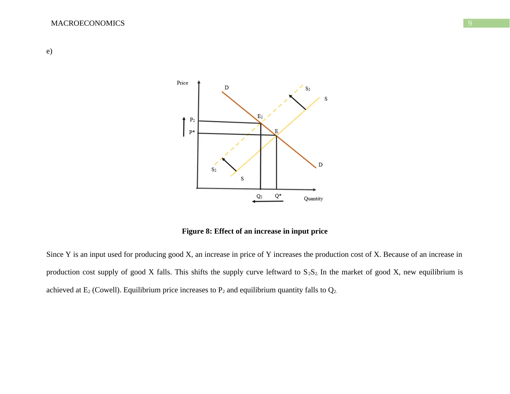
Figure 8: Effect of an increase in input price
Since Y is an input used for producing good X, an increase in price of Y increases the production cost of X. Because of an increase in
production cost supply of good X falls. This shifts the supply curve leftward to S2S2. In the market of good X, new equilibrium is
achieved at E2 (Cowell). Equilibrium price increases to P2 and equilibrium quantity falls to Q2.

10MACROECONOMICS
Question 3
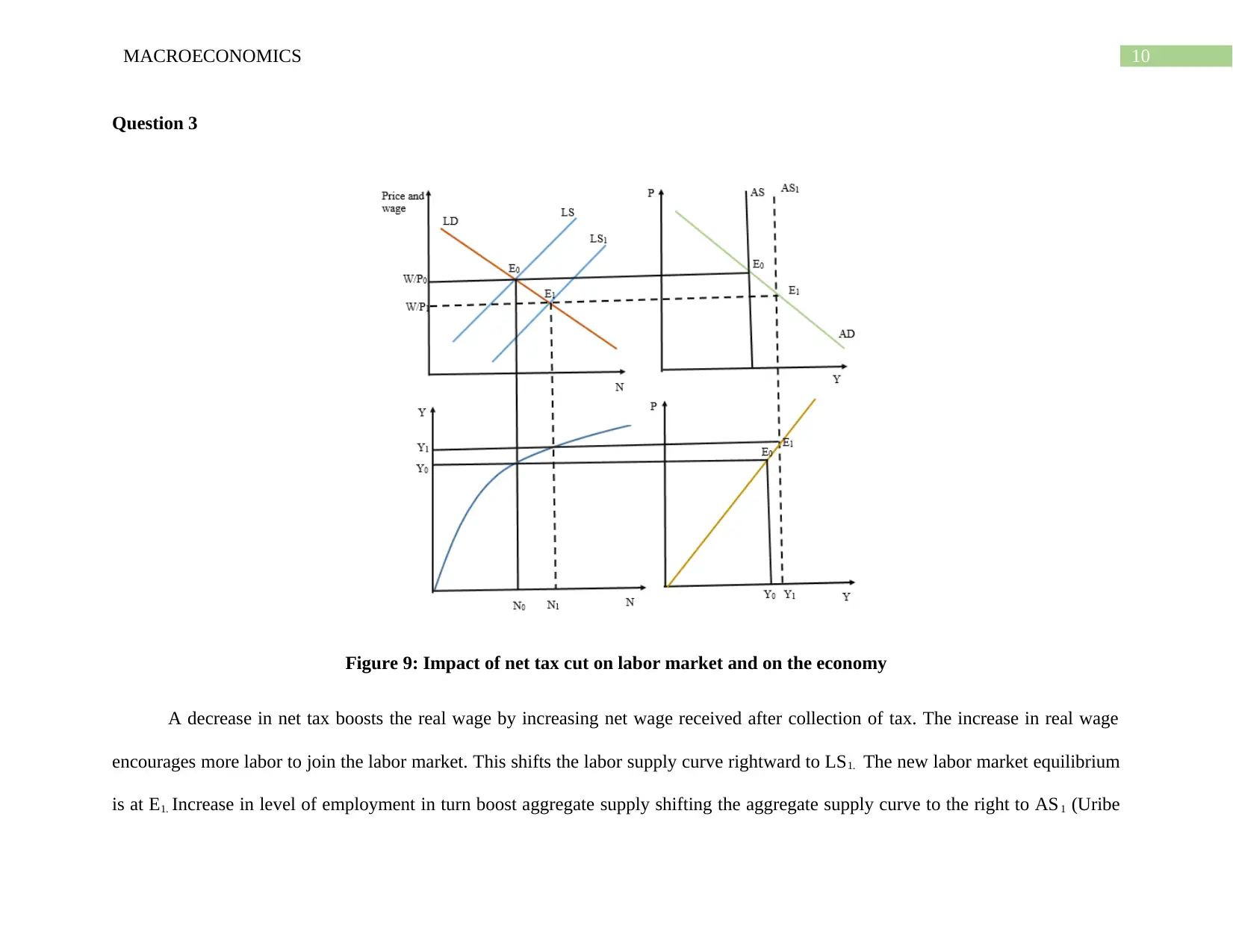
Figure 9: Impact of net tax cut on labor market and on the economy
A decrease in net tax boosts the real wage by increasing net wage received after collection of tax. The increase in real wage
encourages more labor to join the labor market. This shifts the labor supply curve rightward to LS1. The new labor market equilibrium
is at E1. Increase in level of employment in turn boost aggregate supply shifting the aggregate supply curve to the right to AS 1 (Uribe

11MACROECONOMICS
and Schmitt-Grohe). The macroeconomic equilibrium shifts from E to E1. This results in increase in aggregate output of the economy.
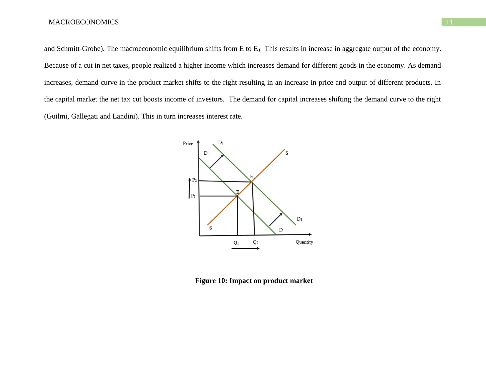
Because of a cut in net taxes, people realized a higher income which increases demand for different goods in the economy. As demand
increases, demand curve in the product market shifts to the right resulting in an increase in price and output of different products. In
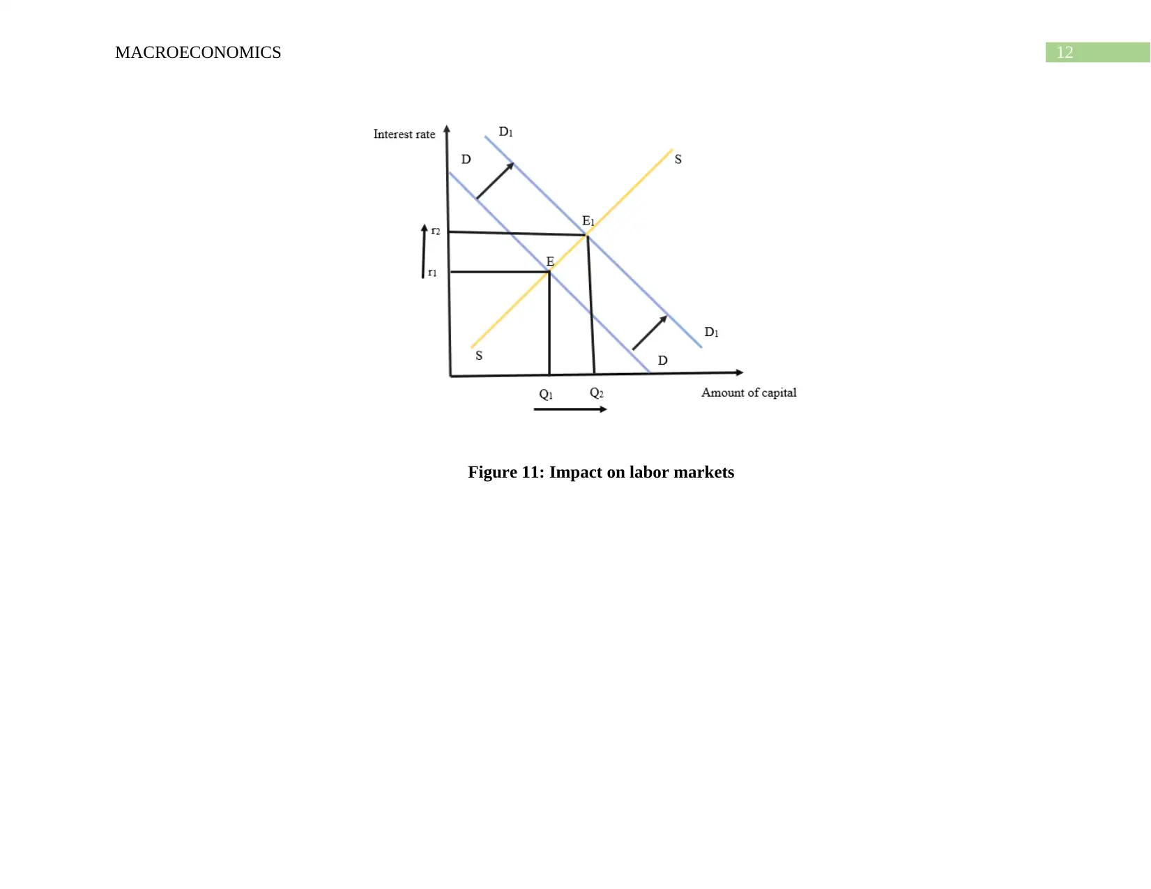
the capital market the net tax cut boosts income of investors. The demand for capital increases shifting the demand curve to the right
(Guilmi, Gallegati and Landini). This in turn increases interest rate.
Figure 10: Impact on product market

12MACROECONOMICS
Figure 11: Impact on labor markets

13MACROECONOMICS
References
Cowell, Frank. Microeconomics: principles and analysis. Oxford University Press, 2018.
Fine, Ben. "Microeconomics." University of Chicago Press Economics Books (2016).
Guilmi, Corrado Di, Mauro Gallegati, and Simone Landini. "Interactive Macroeconomics." Cambridge Books (2017).
Heijdra, Ben J. Foundations of modern macroeconomics. Oxford university press, 2017.
Mankiw, N. Gregory. Principles of microeconomics. Cengage Learning, 2020.
Uribe, Martin, and Stephanie Schmitt-Grohé. Open economy macroeconomics. Princeton University Press, 2017.