Macroeconomics

This document provides a comprehensive study material on Macroeconomics. It covers various topics such as GDP, consumption, investment, government expenditure, net export, fiscal policy, monetary policy, and the impact of trade escalation on the Australian economy. The document also includes solved assignments and references for further reading.

Running head: MACROECONOMICS
Macroeconomics
Name of the student
Name of the university
Course ID

1MACROECONOMICS
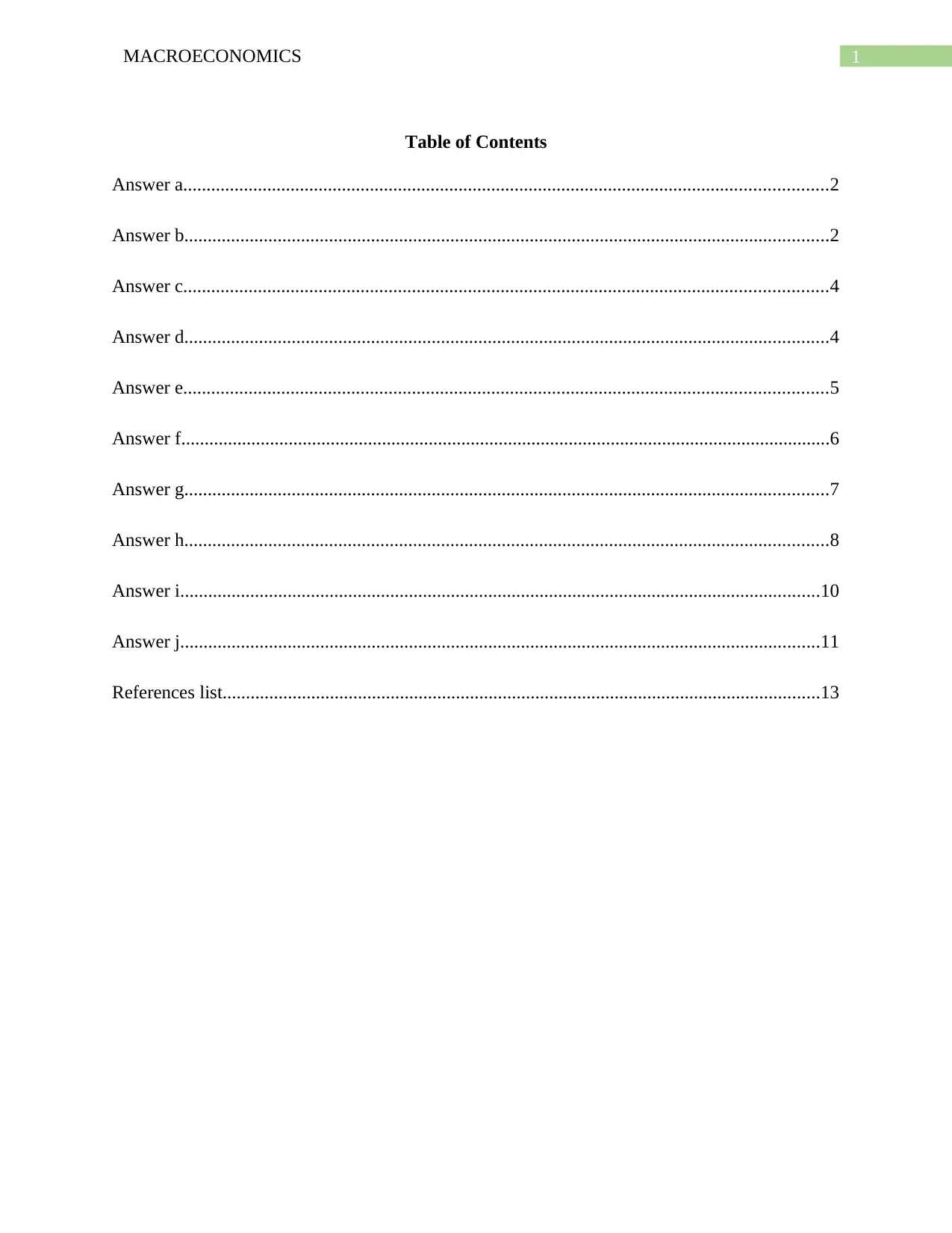
Table of Contents
Answer a..........................................................................................................................................2
Answer b..........................................................................................................................................2
Answer c..........................................................................................................................................4
Answer d..........................................................................................................................................4
Answer e..........................................................................................................................................5
Answer f...........................................................................................................................................6
Answer g..........................................................................................................................................7
Answer h..........................................................................................................................................8
Answer i.........................................................................................................................................10
Answer j.........................................................................................................................................11
References list................................................................................................................................13

2MACROECONOMICS
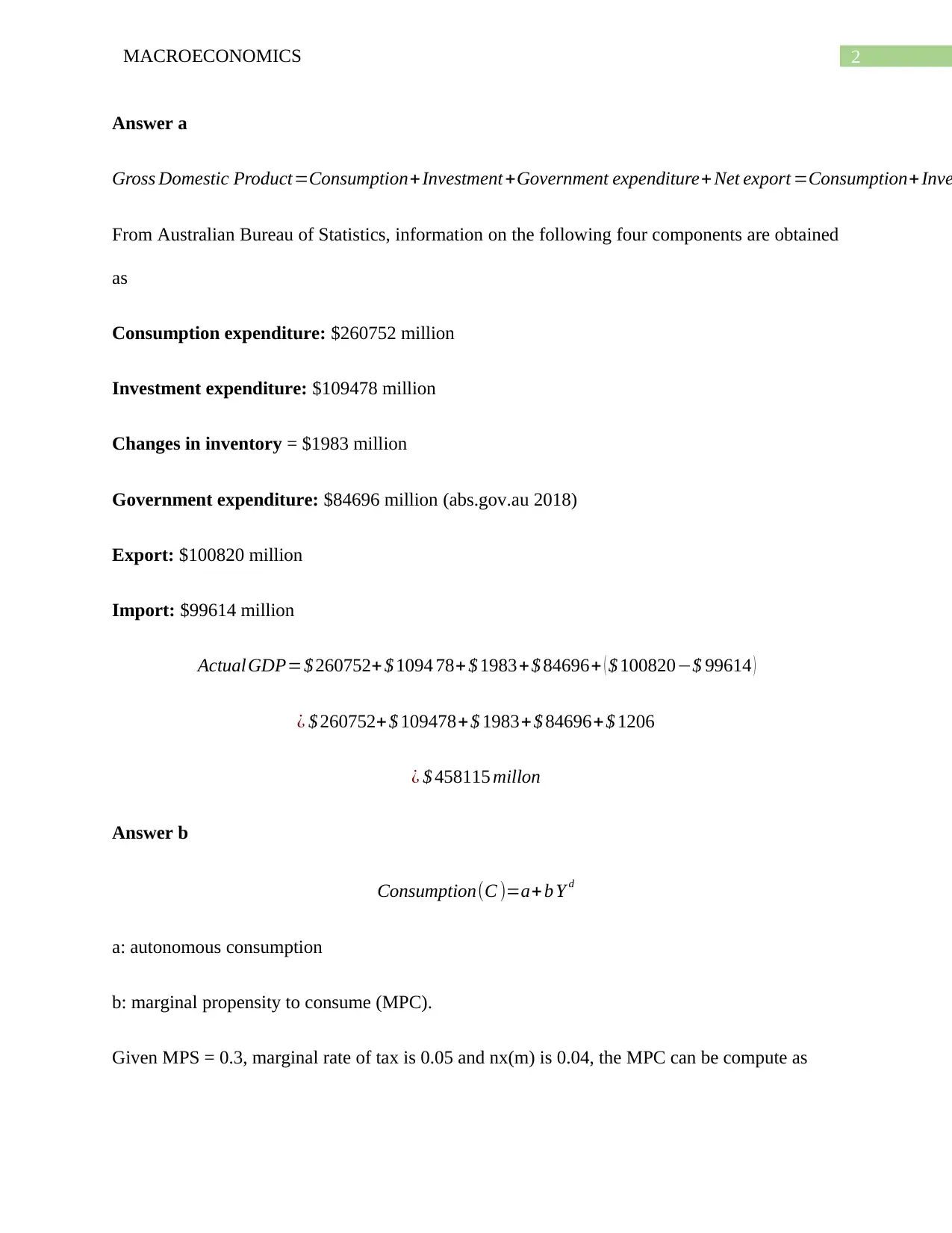
Answer a
Gross Domestic Product=Consumption+Investment +Government expenditure+ Net export =Consumption+ Inve
From Australian Bureau of Statistics, information on the following four components are obtained
as
Consumption expenditure: $260752 million
Investment expenditure: $109478 million
Changes in inventory = $1983 million
Government expenditure: $84696 million (abs.gov.au 2018)
Export: $100820 million
Import: $99614 million
ActualGDP=$ 260752+ $ 1094 78+ $ 1983+$ 84696+ ( $ 100820−$ 99614 )
¿ $ 260752+$ 109478+ $ 1983+$ 84696+ $ 1206
¿ $ 458115 millon
Answer b
Consumption(C )=a+ b Y d
a: autonomous consumption
b: marginal propensity to consume (MPC).
Given MPS = 0.3, marginal rate of tax is 0.05 and nx(m) is 0.04, the MPC can be compute as

3MACROECONOMICS
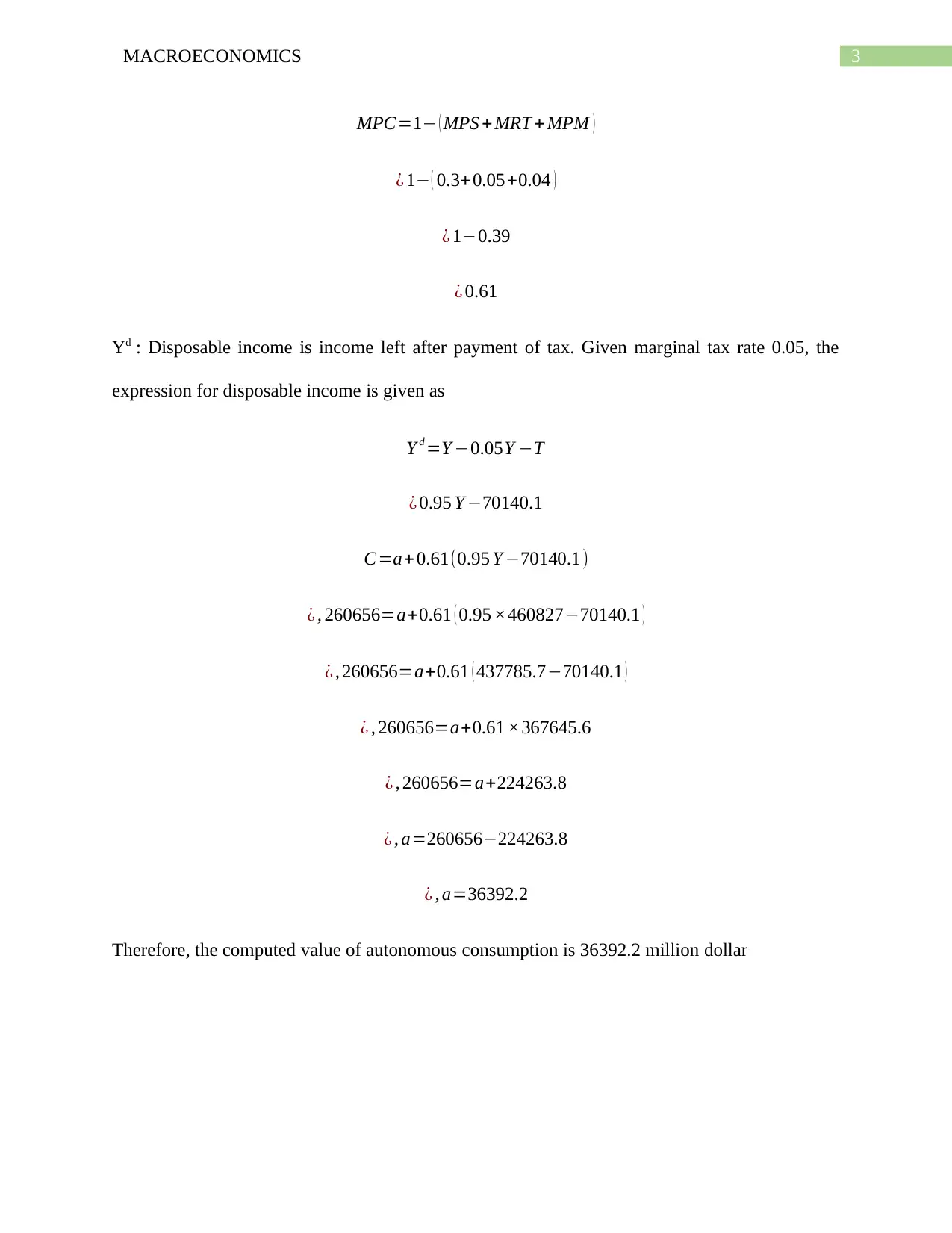
MPC=1− ( MPS +MRT + MPM )
¿ 1− ( 0.3+0.05+0.04 )
¿ 1−0.39
¿ 0.61
Yd : Disposable income is income left after payment of tax. Given marginal tax rate 0.05, the
expression for disposable income is given as
Y d =Y −0.05Y −T
¿ 0.95 Y −70140.1
C=a+ 0.61(0.95 Y −70140.1)
¿ , 260656=a+0.61 ( 0.95 ×460827−70140.1 )
¿ , 260656=a+0.61 ( 437785.7−70140.1 )
¿ , 260656=a+0.61 ×367645.6
¿ , 260656=a+224263.8
¿ , a=260656−224263.8
¿ , a=36392.2
Therefore, the computed value of autonomous consumption is 36392.2 million dollar

4MACROECONOMICS
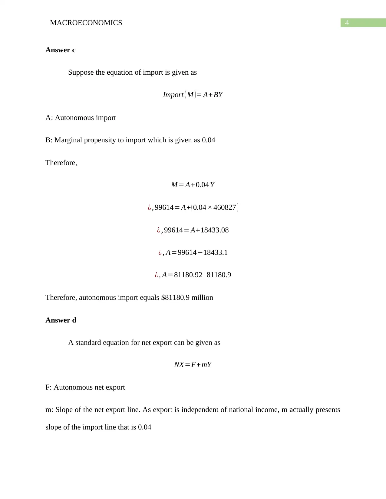
Answer c
Suppose the equation of import is given as
Import ( M )= A+ BY
A: Autonomous import
B: Marginal propensity to import which is given as 0.04
Therefore,
M = A+ 0.04 Y
¿ , 99614= A+ ( 0.04 × 460827 )
¿ , 99614= A+18433.08
¿ , A=99614−18433.1
¿ , A=81180.92 81180.9
Therefore, autonomous import equals $81180.9 million
Answer d
A standard equation for net export can be given as
NX =F+mY
F: Autonomous net export
m: Slope of the net export line. As export is independent of national income, m actually presents
slope of the import line that is 0.04

5MACROECONOMICS
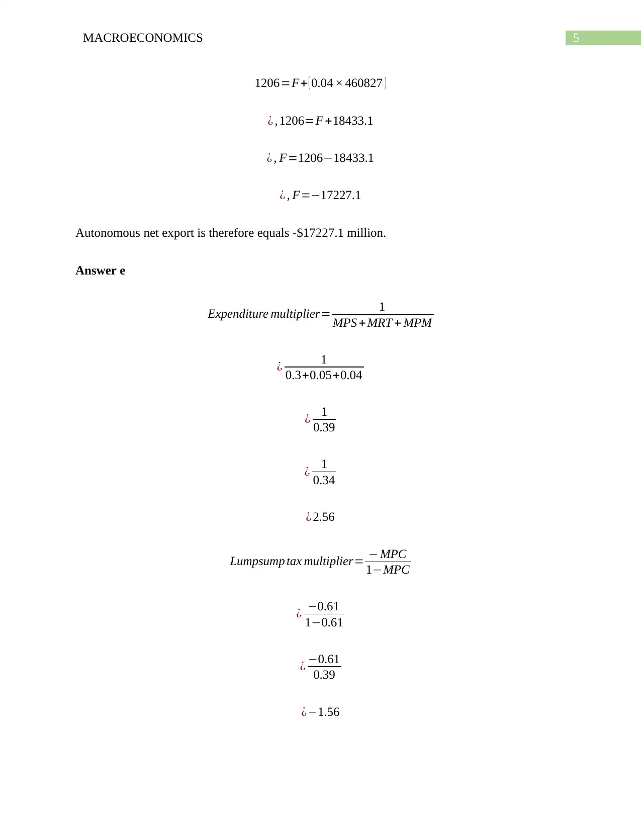
1206=F+ ( 0.04 × 460827 )
¿ , 1206=F +18433.1
¿ , F=1206−18433.1
¿ , F=−17227.1
Autonomous net export is therefore equals -$17227.1 million.
Answer e
Expenditure multiplier= 1
MPS + MRT + MPM
¿ 1
0.3+0.05+0.04
¿ 1
0.39
¿ 1
0.34
¿ 2.56
Lumpsump tax multiplier= − MPC
1−MPC
¿ −0.61
1−0.61
¿ −0.61
0.39
¿−1.56

6MACROECONOMICS
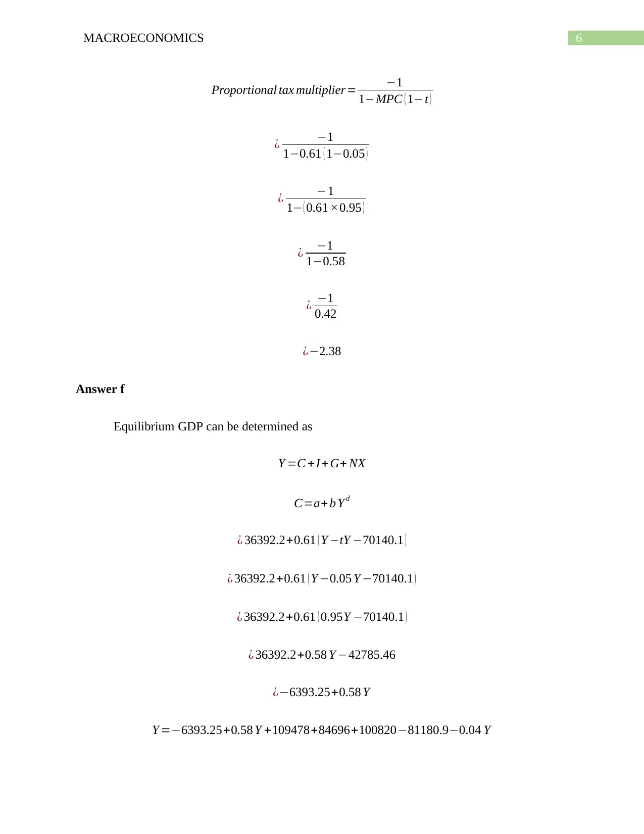
Proportional tax multiplier= −1
1−MPC ( 1−t )
¿ −1
1−0.61 ( 1−0.05 )
¿ −1
1− ( 0.61 ×0.95 )
¿ −1
1−0.58
¿ −1
0.42
¿−2.38
Answer f
Equilibrium GDP can be determined as
Y =C +I+ G+ NX
C=a+ b Y d
¿ 36392.2+0.61 ( Y −tY −70140.1 )
¿ 36392.2+0.61 ( Y −0.05 Y −70140.1 )
¿ 36392.2+0.61 ( 0.95Y −70140.1 )
¿ 36392.2+0.58 Y −42785.46
¿−6393.25+0.58 Y
Y =−6393.25+0.58 Y +109478+84696+100820−81180.9−0.04 Y

7MACROECONOMICS
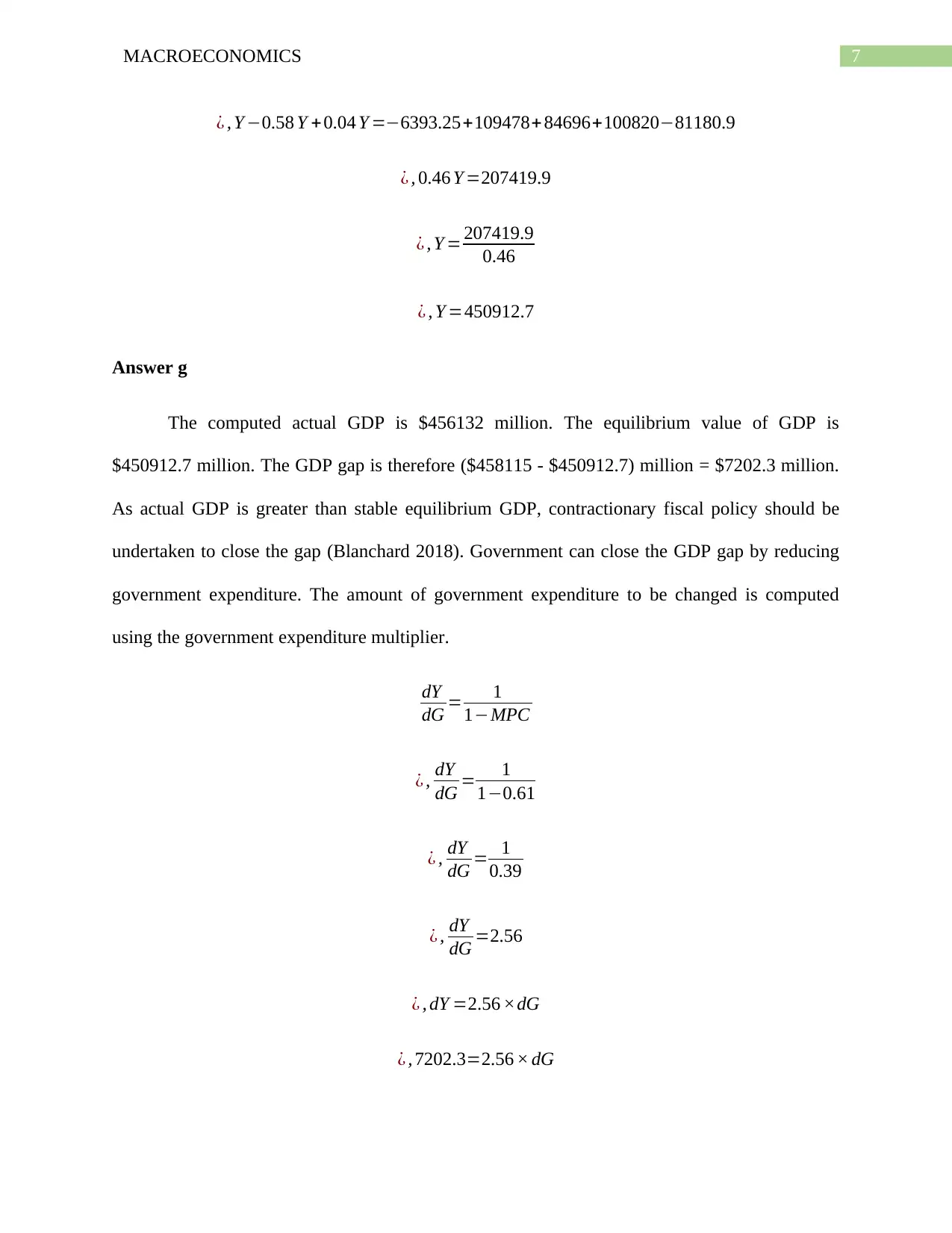
¿ , Y −0.58 Y +0.04 Y =−6393.25+109478+ 84696+100820−81180.9
¿ , 0.46 Y =207419.9
¿ , Y = 207419.9
0.46
¿ , Y =450912.7
Answer g
The computed actual GDP is $456132 million. The equilibrium value of GDP is
$450912.7 million. The GDP gap is therefore ($458115 - $450912.7) million = $7202.3 million.
As actual GDP is greater than stable equilibrium GDP, contractionary fiscal policy should be
undertaken to close the gap (Blanchard 2018). Government can close the GDP gap by reducing
government expenditure. The amount of government expenditure to be changed is computed
using the government expenditure multiplier.
dY
dG = 1
1−MPC
¿ , dY
dG = 1
1−0.61
¿ , dY
dG = 1
0.39
¿ , dY
dG =2.56
¿ , dY =2.56 ×dG
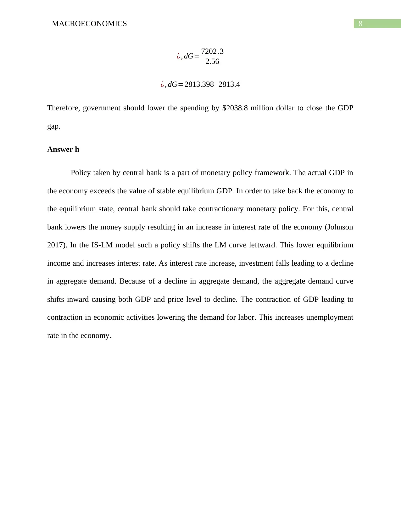
¿ , 7202.3=2.56 × dG

8MACROECONOMICS
¿ , dG= 7202 .3
2.56
¿ , dG=2813.398 2813.4
Therefore, government should lower the spending by $2038.8 million dollar to close the GDP
gap.
Answer h
Policy taken by central bank is a part of monetary policy framework. The actual GDP in
the economy exceeds the value of stable equilibrium GDP. In order to take back the economy to
the equilibrium state, central bank should take contractionary monetary policy. For this, central
bank lowers the money supply resulting in an increase in interest rate of the economy (Johnson
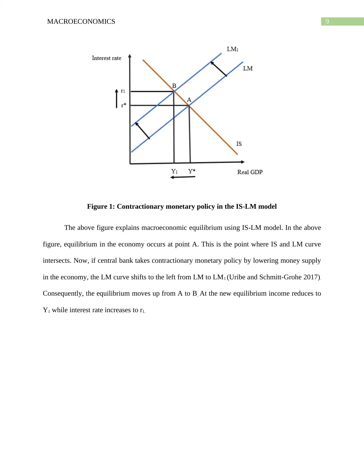
2017). In the IS-LM model such a policy shifts the LM curve leftward. This lower equilibrium
income and increases interest rate. As interest rate increase, investment falls leading to a decline
in aggregate demand. Because of a decline in aggregate demand, the aggregate demand curve
shifts inward causing both GDP and price level to decline. The contraction of GDP leading to
contraction in economic activities lowering the demand for labor. This increases unemployment
rate in the economy.

9MACROECONOMICS
Figure 1: Contractionary monetary policy in the IS-LM model
The above figure explains macroeconomic equilibrium using IS-LM model. In the above
figure, equilibrium in the economy occurs at point A. This is the point where IS and LM curve
intersects. Now, if central bank takes contractionary monetary policy by lowering money supply
in the economy, the LM curve shifts to the left from LM to LM1 (Uribe and Schmitt-Grohe 2017).
Consequently, the equilibrium moves up from A to B. At the new equilibrium income reduces to
Y1 while interest rate increases to r1.

10MACROECONOMICS
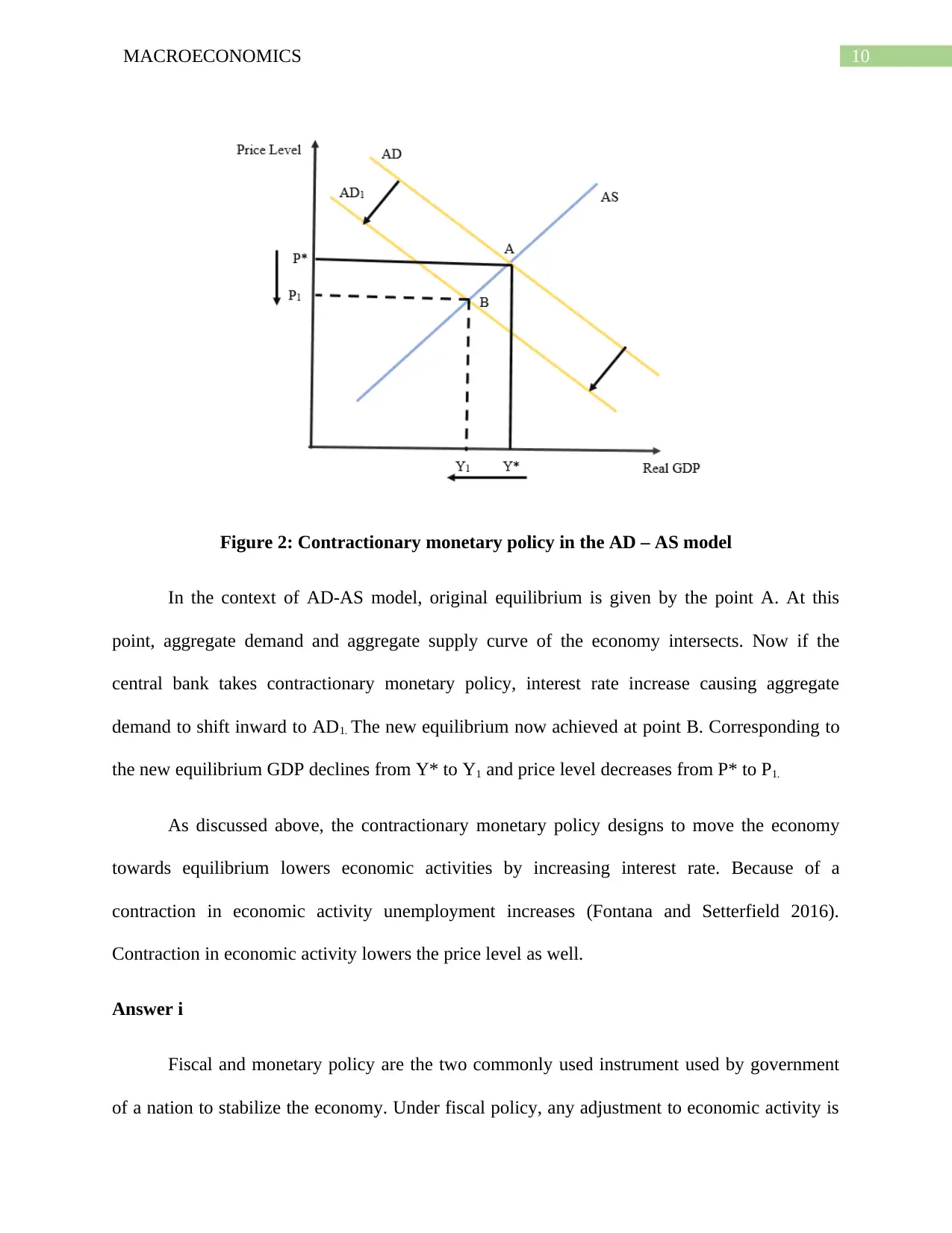
Figure 2: Contractionary monetary policy in the AD – AS model
In the context of AD-AS model, original equilibrium is given by the point A. At this
point, aggregate demand and aggregate supply curve of the economy intersects. Now if the
central bank takes contractionary monetary policy, interest rate increase causing aggregate
demand to shift inward to AD1. The new equilibrium now achieved at point B. Corresponding to
the new equilibrium GDP declines from Y* to Y1 and price level decreases from P* to P1.
As discussed above, the contractionary monetary policy designs to move the economy
towards equilibrium lowers economic activities by increasing interest rate. Because of a
contraction in economic activity unemployment increases (Fontana and Setterfield 2016).
Contraction in economic activity lowers the price level as well.
Answer i
Fiscal and monetary policy are the two commonly used instrument used by government
of a nation to stabilize the economy. Under fiscal policy, any adjustment to economic activity is

11MACROECONOMICS
done by changing either government spending or tax. Under money policy, central bank of a
nation influences economic activity by changing money supply or interest rate. Traditionally,
monetary policy has some potential benefit over fiscal policy. The first advantage of monetary
policy is that targeted policy is designed by the monetary authorities that are politically neutral
(Heijdra 2017). The purpose and objectives of central banks are different from that of state
government. For this, money policy results in an unbiased policy design for the nation leading to
more successful accomplishment of objectives like stable growth, high employment and stability
in price level. Another benefits of using monetary policy is that money policy does not contribute
to budget deficit. Under fiscal policy there is a substantial tendency to overspend resulting in a
budget deficit and thus constraints government’s capacity to provide stimulus to the economy
during recession (Mankiw 2014). Another disadvantage of fiscal policy is that increase in
government spending crowd out private investment which is unlikely to happen in case of
monetary policy.
Answer j
The trade escalation between US and China and spread to the global economy likely to
have a potentially significant impact on a mid-sized economy like Australia. Australian economy
is largely dependent on China’s economy and thus is exposed to a high risk because of trade
disputes between US and China. US-China trade war will cause China’s economy to contract by
limiting China’s export market (abc.net.au 2018). The economic contraction in China in turn
reduces export demand for Australia. As found by KPMG report an all-out trade in which all
countries increased tariff will cause Australian economy to contract resulting in loss of many
jobs. This will increase unemployment percentage in the economy. As a result of trade
escalation, there is a likely decline in value of Australian dollar causing import prices to increase.

12MACROECONOMICS
Weaker dollar, higher unemployment and high price will make Australian household worse-off.
On the other side, there are some sectors that may be benefitted from tariff retaliation between
China and US. One such sector agribusiness in Australia (pwc.com.au 2018). Demand of
Australian grains and wines may increase if China retaliates against imports from US. Other
sectors like Steel and LNG businesses may also be placed in a potential advantageous position in
case tariffs are imposed on China’s or US’s product.

13MACROECONOMICS
References list
abc.net.au 2018. Trump's trade war could wipe billions from Australia's economy. [online] ABC
News. Available at: https://www.abc.net.au/news/2018-04-09/trade-war-could-wipe-billions-
from-australian-economy/9633176 [Accessed 12 May 2019].
abs.gov.au 2018. 5206.0 - Australian National Accounts: National Income, Expenditure and
Product, Dec 2018. [online] Abs.gov.au. Available at:
https://www.abs.gov.au/AUSSTATS/abs@.nsf/DetailsPage/5206.0Dec%202018?
OpenDocument [Accessed 12 May 2019].
Blanchard, O., 2018. On the future of macroeconomic models. Oxford Review of Economic
Policy, 34(1-2), pp.43-54.
Fontana, G. and Setterfield, M. eds., 2016. Macroeconomic theory and macroeconomic
pedagogy. Springer.
Heijdra, B.J., 2017. Foundations of modern macroeconomics. Oxford university press.
Johnson, H.G., 2017. Macroeconomics and monetary theory. Routledge.
Mankiw, N.G., 2014. Brief principles of macroeconomics. Cengage Learning.
pwc.com.au 2018. US-China trade war not all bad for Australia. [online] PwC. Available at:
https://www.pwc.com.au/press-room/2018/us-china-trade-war-not-all-bad-for-australia.html
[Accessed 12 May 2019].
Uribe, M. and Schmitt-Grohe, S., 2017. Open economy macroeconomics. Princeton University
Press.