Management Economics Question 2022

1Management Economics
Running head: MANAGEMENT ECONOMICS
Management Economics
Author’s Name
Institutional Affiliation

2Management Economics
Management Economics
Question 1
(i) Hypothetical Demand Function
(a) Selection of Explanatory Variables in the Function. Law of Demand
depicts that whenever price of a certain commodity falls, the consumers tend to buy
more and vice versa (The Economic Times, 2019). The variables include the annual
income of consumers, their preferences, and the prices of other substitute or competitive
products in the market. The equation which holds the relations of all the influencers is
recognized by demand function by the economists. It can thus, be explained through a
simpler linear equation as provided below:
Qdx = f (Px, I, Py,…..)……………………………………………….. (1)
Where;
Qdx = Quantitative Demand for Good X
Px = Price per Unit of the commodity X
Py = Price per Unit of the subsidiary product Y.
I = income of the consumer (as in $1000 per household annually)
The equation describes that quantity demanded of commodity X is dependent on the
summarized price of Commodity X, Y and the income of the consumer as well as other
variables. The following linear equation describes tea consumption of a small town’s
per-household per week, whereas Py might be the average price of sugar used in $1,000
Qdx= 6.8-0.2 Px + 0.072 -0.01 Py ……………………………………….. (2)
The exemplified equation above depicts that tea consumption gets reduced with
rise in the price of sugar.This kind of definite relationship indicate the existence of
negative cross-price elasticity of demand between the tea and sugar (complementary
products) (Eastin & Arbogast, 2011).
(b) Demand Elasticities. Theory of Elasticity is a microeconomic factors, as per
which the change in one variable brings about an alteration in the value of another

3Management Economics
variable. In this case, the price of a good cannot be considered as the only functional
determinant of quantity demanded, as it also relies on the factor of consumer income
(Economics Online, 2019).
Own price elasticity is the major influencer, which helps in determining the concept of
normal goods and inferior goods. It is explained by the Law of demand that own-price
elasticity of demand will almost always be negative but the income elasticity can be
negative, positive, or zero. The negative impact of the income can further be understood
from the fact that a sudden rise in exogenous income reduces the consumption level of
the customers to a large extent. This can be more clearly inferred from the example of
inferior goods, which precisely highlights that there exists an inverse relationship
between the factors of quantity demanded and consumer income (Nechyba, 2011).
The variable in the right-hand side of the demand function acts as the basis of its
own demand. When the price of other commodity creates an impact on the demand of
another commodity, it is generally identified as cross-price elasticity of demand.
Through this concept, substitutes and complements can be adequately described. For
instance, in case of some series of goods P and Q, when the price of ‘P’ rises and
demand for Q automatically increases, this situation is known to be positive cross
elasticity of demand and the commodities are defined as substitutes. On the contrary,
complementary goods refer to those two products, where fall in the price of one
commodity leads to the rise in the demand for the other. Such a scenario can be termed
as Negative Cross-Price Elasticity of Demand (Xplaind, 2019). The previously
discussed equation provides us with the knowledge of negative cross elasticity, as the
goods are inclined to be consumed together as a pair. However, the determination of
substitutes and complements can be determined through instant surveillance and
statistical analysis (Shocker, Bayus & Kim, 2015).
(ii) Demand for Electricity
(a) Profit Maximizing Amounts. In order to maximize profit, the firm requires
MC=MR (Agarwal, 2019)
The profit demand function is P=1200-4Q
Total production is Q = Q1 + Q2 and the cost of producing electricity are provided by
C1(Q1).

4Management Economics
Explanation: It can thus, be perceived that,
MR= 1200-8Q, MC1= 12Q1
MC2= 6Q2
It can be also written as MR = MC1and MR =MC2. Since, (Q = Q1 + Q2) is
given, therefore it can be written
1200 – 8(Q1+ Q2) = 12Q1………………………………………………. (1)
1200 – 8(Q1+ Q2) = 6Q2………………………………………………… (2)
By solving the equation we can get Q1 = 33.33 and Q2 = 66.67. The optimal price
is considered by the amount, which is paid by the consumers for the Q1+ Q2= 100 units
which have been further determined by the inverse demand curve;
P = 1200 – 4(100) = $800.
At this price and output, revenues can be described by
R = ($800)*(100) = $80,000.00
While the costs are C1+ C2= (8,000 + 6(33.33)2) + (6,000 + 3(66.67)2) =
$34,000.
Therefore, the firm will earn the profits of $46,000.00.
(b) Optimal Price. The optimal price can be determined through
Q1+ Q2= 100
Since, Q1 = 33.33
Q2 = 66.67,
The optimal price will be 33.33+66.67=100 Or 1
(c) Optimal Quantity. Since MR=MC2
1200-8(Q1+ Q2) = 6Q2
8Q1+14 Q2 =1200

5Management Economics
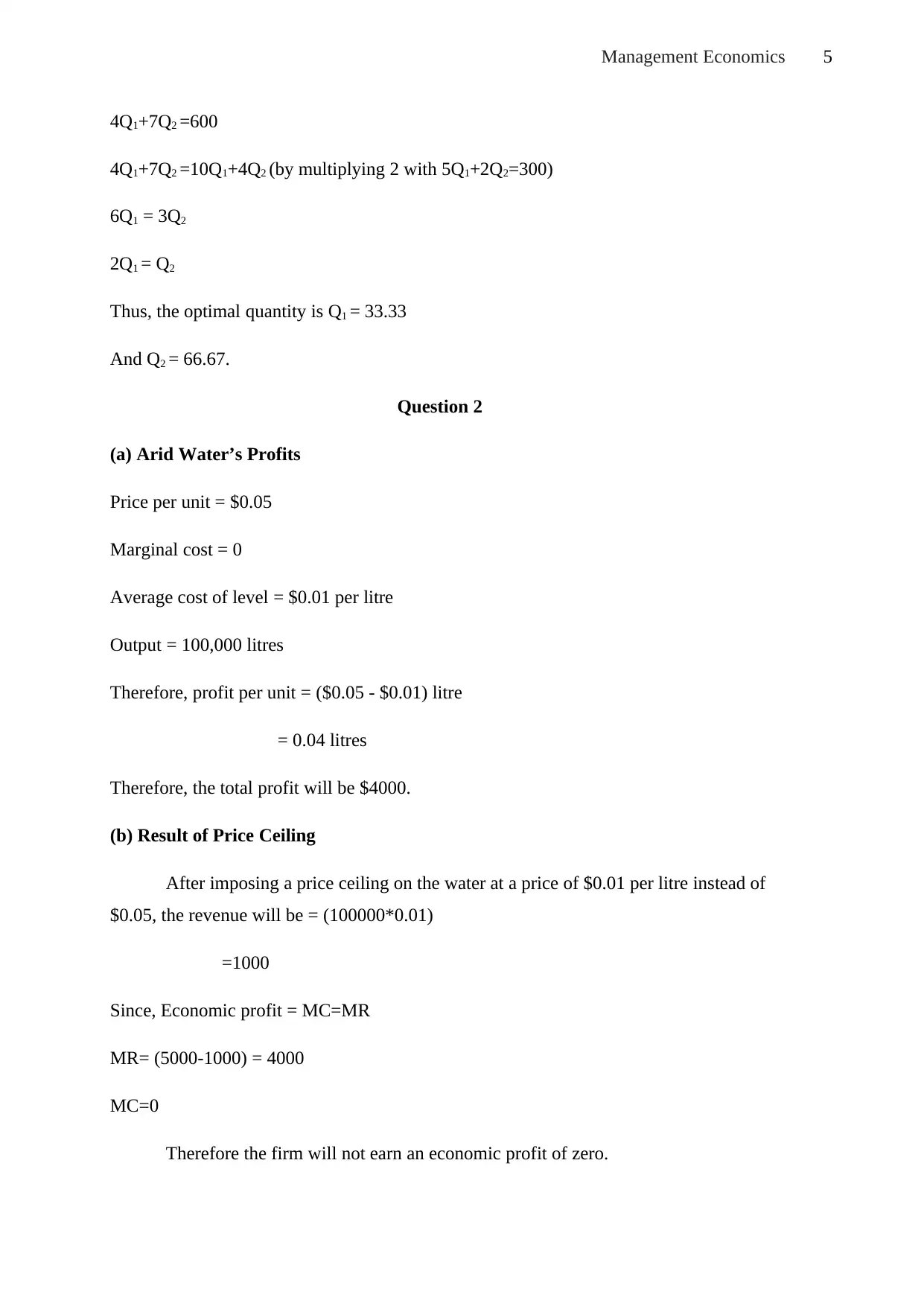
4Q1+7Q2 =600
4Q1+7Q2 =10Q1+4Q2 (by multiplying 2 with 5Q1+2Q2=300)
6Q1 = 3Q2
2Q1 = Q2
Thus, the optimal quantity is Q1 = 33.33
And Q2 = 66.67.
Question 2
(a) Arid Water’s Profits
Price per unit = $0.05
Marginal cost = 0
Average cost of level = $0.01 per litre
Output = 100,000 litres
Therefore, profit per unit = ($0.05 - $0.01) litre
= 0.04 litres
Therefore, the total profit will be $4000.
(b) Result of Price Ceiling
After imposing a price ceiling on the water at a price of $0.01 per litre instead of
$0.05, the revenue will be = (100000*0.01)
=1000
Since, Economic profit = MC=MR
MR= (5000-1000) = 4000
MC=0
Therefore the firm will not earn an economic profit of zero.

6Management Economics
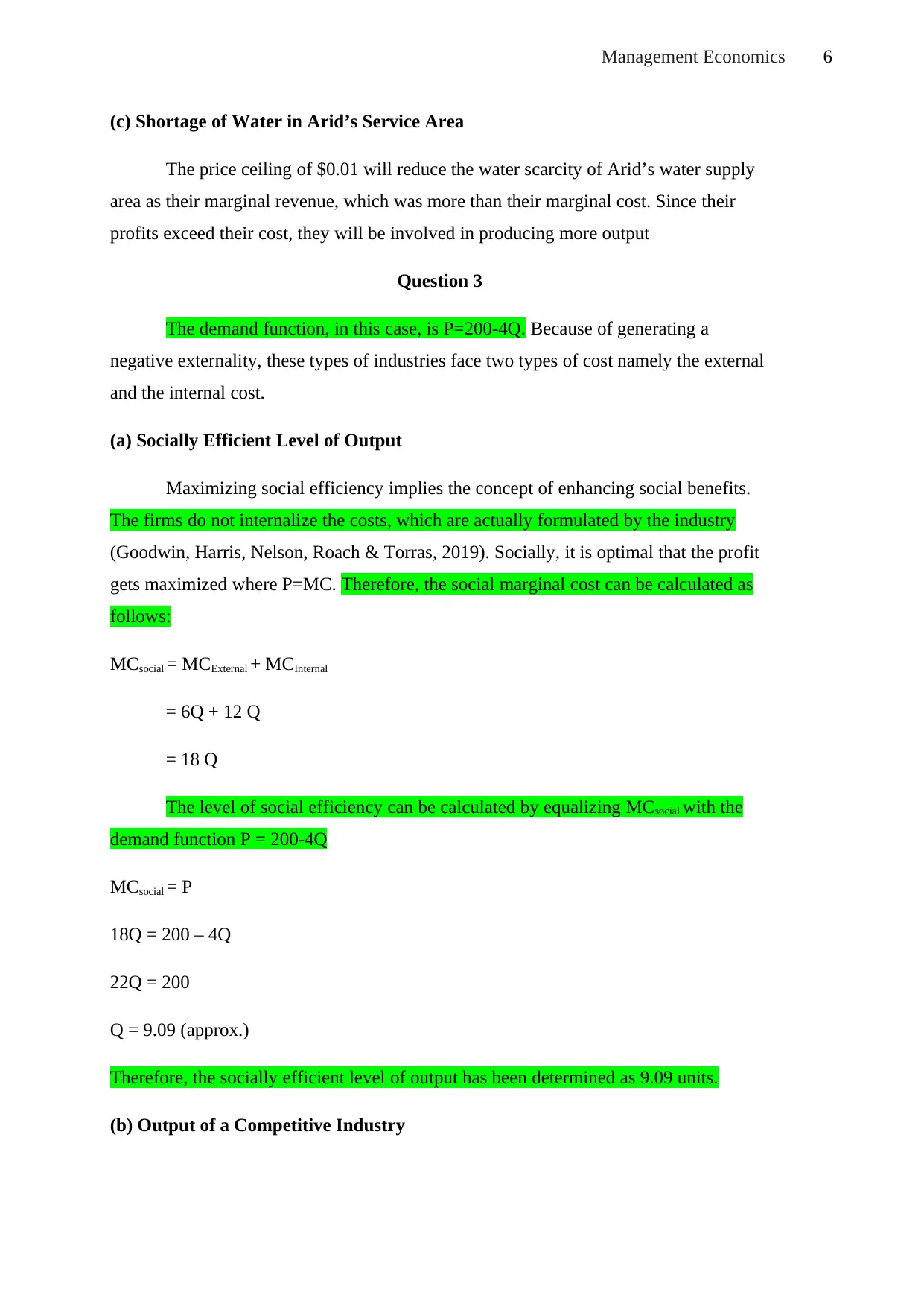
(c) Shortage of Water in Arid’s Service Area
The price ceiling of $0.01 will reduce the water scarcity of Arid’s water supply
area as their marginal revenue, which was more than their marginal cost. Since their
profits exceed their cost, they will be involved in producing more output
Question 3
The demand function, in this case, is P=200-4Q. Because of generating a
negative externality, these types of industries face two types of cost namely the external
and the internal cost.
(a) Socially Efficient Level of Output
Maximizing social efficiency implies the concept of enhancing social benefits.
The firms do not internalize the costs, which are actually formulated by the industry
(Goodwin, Harris, Nelson, Roach & Torras, 2019). Socially, it is optimal that the profit
gets maximized where P=MC. Therefore, the social marginal cost can be calculated as
follows:
MCsocial = MCExternal + MCInternal
= 6Q + 12 Q
= 18 Q
The level of social efficiency can be calculated by equalizing MCsocial with the
demand function P = 200-4Q
MCsocial = P
18Q = 200 – 4Q
22Q = 200
Q = 9.09 (approx.)
Therefore, the socially efficient level of output has been determined as 9.09 units.
(b) Output of a Competitive Industry

7Management Economics
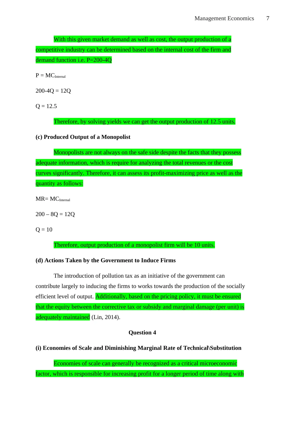
With this given market demand as well as cost, the output production of a
competitive industry can be determined based on the internal cost of the firm and
demand function i.e. P=200-4Q
P = MCInternal
200-4Q = 12Q
Q = 12.5
Therefore, by solving yields we can get the output production of 12.5 units.
(c) Produced Output of a Monopolist
Monopolists are not always on the safe side despite the facts that they possess
adequate information, which is require for analyzing the total revenues or the cost
curves significantly. Therefore, it can assess its profit-maximizing price as well as the
quantity as follows:
MR= MCInternal
200 – 8Q = 12Q
Q = 10
Therefore, output production of a monopolist firm will be 10 units.
(d) Actions Taken by the Government to Induce Firms
The introduction of pollution tax as an initiative of the government can
contribute largely to inducing the firms to works towards the production of the socially
efficient level of output. Additionally, based on the pricing policy, it must be ensured
that the equity between the corrective tax or subsidy and marginal damage (per unit) is
adequately maintained (Lin, 2014).
Question 4
(i) Economies of Scale and Diminishing Marginal Rate of Technical\Substitution
Economies of scale can generally be recognized as a critical microeconomic
factor, which is responsible for increasing profit for a longer period of time along with

8Management Economics
maintaining the economy to support the entire business (Kumar, 2019). An economy of
scale intends to describe the increasing output rate and decreasing average cost in the
long term and the firm’s efficiency is affected by the size of the firm (Economics Online
a, 2019).
(ii) Hiring a Worker
(a) Highest Annual Salary Payable. Hiring additional worker will increase the
firm’s output by 2000 units, which will further lead towards an increase in the marginal
product level (MPL) for the extra worker i.e. 2000
Price of output = $20
So, the highest salary, I would be eager to pay is equal to MPL multiplied by price.
Therefore, Maximum wage = 2000 x $40 = $80,000
(b) Need of Paying High Amount. It can be determined by the market wage
rate. If the market wage rate is higher than $80,000, this worker will reject my offer
because he could get paid more than that from another company. If the market wage is
lower than $80,000 then the worker will accept my offer but I would have to incur an
operating loss by offering a worker privileged salary than the competitors are paying.

9Management Economics
References
Agarwal, P. (Jun 30, 2019). Profit maximization rule formula. Retrieved September 21,
2019, from https://www.intelligenteconomist.com/profit-maximization-rule/
Anwar, R.S., & Ali, S. (2015). Economies of Scale. International Interdisciplinary
Journal of Scholarly Research, 1(1), 51-57.
Eastin, R.V., & Arbogast, G.L. (2011).Demand and Supply Analysis: Introduction. CFA
Institute, 2-55.
Economics Online a.(2019). Economies of scale. Retrieved September 21, 2019, from
https://www.economicsonline.co.uk/Business_economics/Economies_of_scale.ht
ml
Economics Online. (2019). Elasticity. Retrieved September 21, 2019, from
https://www.economicsonline.co.uk/Competitive_markets/Elasticity.html
Goodwin, N., Harris, J.M., Nelson, J.A., Roach, B., & Torras, M. (2019). Principles of
Economics in Context. United Kingdom, UK: Routledge
Kumar, S. (2018, August 17). How to Defend the Economies of Scale. Retrieved
September 21, 2019, from https://www.valuewalk.com/2018/08/market-share-
moat/
Lin, S.A.Y. (2014). Theory and Measurement of Economic Externalities. United States,
US: Academic Press
Nechyba, T. (2011). Microeconomics: an intuitive approach with calculus. United
States, US: Cengage Learning.
Shocker, A.D., Bayus, B. L., & Kim, N. (2015). Product complements and substitutes in
the real world:the relevance of “other products”. Journal of Marketing, 1-40.
The Economic Times. (2019). Definition of 'Law of Demand'. Retrieved September 21,
2019, from https://economictimes.indiatimes.com/definition/law-of-demand
Xplaind. (2019). Substitute Vs Complements. Retrieved September 21, 2019, from
https://xplaind.com/679438/substitute-vs-complementary-goods