MANAGERIAL ECONOMICS.

Running head: MANAGERIAL ECONOMICS
Managerial Economics
Name of the Student:
Name of the University:
Author Note:

1
MANAGERIAL ECONOMICS
Table of Contents
Introduction................................................................................................................................2
Answer 1....................................................................................................................................2
a.Supply Schedule..................................................................................................................2
Factors affecting supply of a good.........................................................................................2
b. Inelastic demand and change in supply..............................................................................4
Answer 2:...................................................................................................................................5
Degrees of Price Elasticity:....................................................................................................5
Point Elasticity Method:.........................................................................................................6
Answer 4:...................................................................................................................................9
a.Lower cost of vanilla ice cream and effect on chocolate ice crea.......................................9
b.Midwest drought and effect on chocolate ice cream market...............................................9
Answer 5:.................................................................................................................................10
a.Market for newspaper........................................................................................................10
b. Market for St. Louis Rams (a professional football team) cotton T-shirts......................12
d. The market for the Krugman and Wells economics textbook..........................................15
Answer 6:.................................................................................................................................16
a.Equilibrium in the rose market..........................................................................................16
b.Comparative advantage in rose production.......................................................................17
c.Domestic production and import of rose under free trade.................................................17
Answer 7:.................................................................................................................................18
a.Market structure of telecommunication market................................................................18
b.Expected pricing strategies in the industry.......................................................................18
Conclusion................................................................................................................................19
References................................................................................................................................20

2
MANAGERIAL ECONOMICS
Introduction
The paper briefly discusses different concepts related to the field of microeconomics.
The areas of focus include supply, demand, equilibrium, demand elasticity, market structure,
and associated pricing strategies.
Answer 1
a.Supply Schedule
Supply schedule refers to a tabular representation of price and corresponding quantity
supplied of a good. There are a number of factors, which can affect the supply schedule and
the supply in the market. Usually, supply depends on the price, the cost of production and
technology (Kreps 2019). An increase (decrease) in supply means there is a rightward
(leftward) shift of supply curve.
Factors affecting supply of a good
A few factors affecting supply are described as follows:
Price:
Price of the product is one of the major factors that affect the supply of a product. A
rise in the price of the product increases the supply of the product and vice versa. A
speculation of future price can also affect the supply, as there is a chance of earning or losing
profit for the seller. If there is speculation of rise in future price, supply of that product will
fall in the resent market.

3
MANAGERIAL ECONOMICS
Technology:
The supply of a product will increase by the introduction of better and advance
technology. Other things remaining same, an advance technology will increase the
production. This results in an increase in supply of the product. For an example, replacement
of old machineries with advance machineries in the factory increases the production.
Input Prices:
The inputs are raw materials, machines, land and equipment, which are used at the
time of production. If there is an increase in factor prices, supply will fall. A rise in inputs
prices will increase the cost of production, which will reduce the supply of product.
Availability of inputs also affects the supply of a product. For example, the labour cost and
transport cost will be less if labour and raw materials are available near the factory (Cowen
and Tabarrok 2015). A reduction in cost will raise the production and supply of the product.
Number of sellers
Number of seller is positively related with market supply. That means larger the
number of sellers in the market higher is the quantity supplied. The accumulated supply of
individual sellers increases market supply.
Expectation
Expectation about future price affects market supply of a good. Events leading to
expectation of a higher price in future induce sellers to reduce current supply. Sellers then
save more inventories to sell their goods at a higher price in future. In contrast, current supply
increases if sellers expect a lower price in future.

4
MANAGERIAL ECONOMICS
Q
Price
Quantity
D
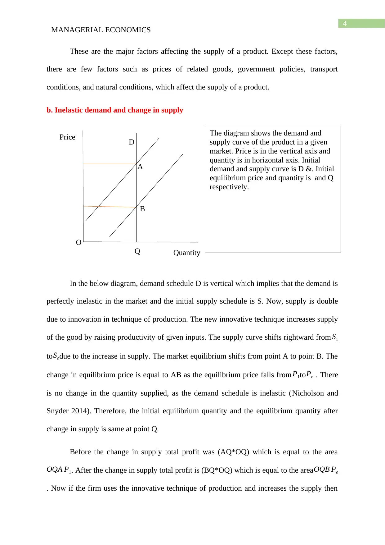
The diagram shows the demand and
supply curve of the product in a given
market. Price is in the vertical axis and
quantity is in horizontal axis. Initial
demand and supply curve is D &. Initial
equilibrium price and quantity is and Q
respectively.
A
B
O
These are the major factors affecting the supply of a product. Except these factors,
there are few factors such as prices of related goods, government policies, transport
conditions, and natural conditions, which affect the supply of a product.
b. Inelastic demand and change in supply
In the below diagram, demand schedule D is vertical which implies that the demand is
perfectly inelastic in the market and the initial supply schedule is S. Now, supply is double
due to innovation in technique of production. The new innovative technique increases supply
of the good by raising productivity of given inputs. The supply curve shifts rightward from S1
to Sedue to the increase in supply. The market equilibrium shifts from point A to point B. The
change in equilibrium price is equal to AB as the equilibrium price falls from P1toPe . There
is no change in the quantity supplied, as the demand schedule is inelastic (Nicholson and
Snyder 2014). Therefore, the initial equilibrium quantity and the equilibrium quantity after
change in supply is same at point Q.
Before the change in supply total profit was (AQ*OQ) which is equal to the area
OQA P1. After the change in supply total profit is (BQ*OQ) which is equal to the area OQB Pe
. Now if the firm uses the innovative technique of production and increases the supply then

5
MANAGERIAL ECONOMICS
the firm has to face a decline in profit, which is equal to the area (
OQA P1−OQB Pe=P1 Pe BA). So, increment in the supply cannot be recommended to the
firm (Blad and Keiding 2014). However, the firm can use the innovative technique of
production to reduce the cost of production not to increase the supply.
Answer 2:
The three common used measure of elasticity of demand are price elasticity of
demand, income elasticity of demand and cross price elasticity of demand (Mahanty 2014).
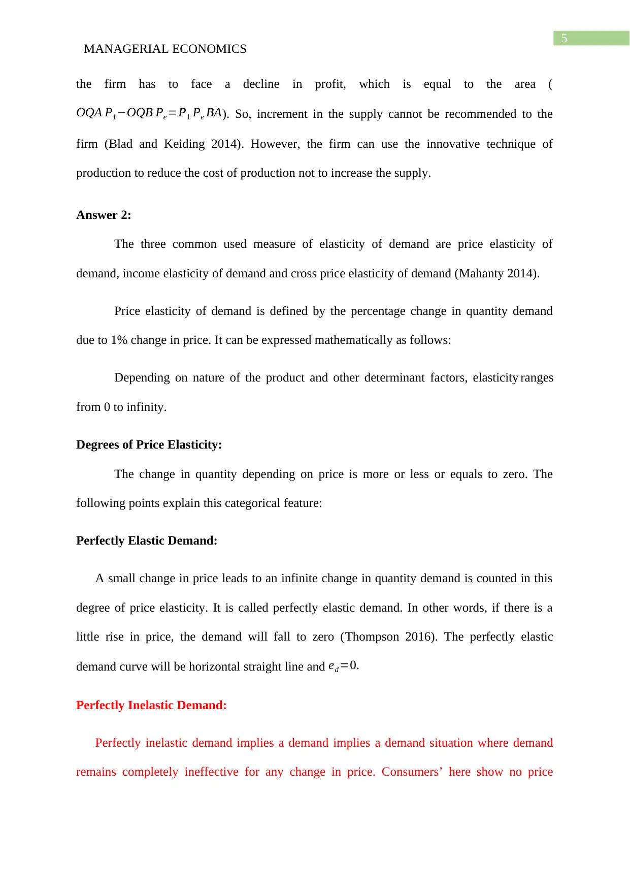
Price elasticity of demand is defined by the percentage change in quantity demand
due to 1% change in price. It can be expressed mathematically as follows:
Depending on nature of the product and other determinant factors, elasticity ranges
from 0 to infinity.
Degrees of Price Elasticity:
The change in quantity depending on price is more or less or equals to zero. The
following points explain this categorical feature:
Perfectly Elastic Demand:
A small change in price leads to an infinite change in quantity demand is counted in this
degree of price elasticity. It is called perfectly elastic demand. In other words, if there is a
little rise in price, the demand will fall to zero (Thompson 2016). The perfectly elastic
demand curve will be horizontal straight line and ed =0.
Perfectly Inelastic Demand:
Perfectly inelastic demand implies a demand implies a demand situation where demand
remains completely ineffective for any change in price. Consumers’ here show no price

6
MANAGERIAL ECONOMICS
sensitivity. The value of demand elasticity is zero. The corresponding demand curve is a
vertical straight line at the fixed quantity.
Unitary Elastic Demand:
There will be a same proportionate change in quantity demand due to a given proportionate
change in price. This is called unitary elastic demand. Simply, proportionate change in price
is equal to the proportionate change in demand. The unitary elastic demand curve will be
rectangular hyperbola and ed =1.
Relatively Elastic Demand:
There will be a relatively big change in quantity demand due to a small change in price.
This is called relatively elastic demand (Stoneman, Bartolon and Baussola 2018). In this case,
change in price has a greater impact on quantity demand. The relatively elastic demand curve
is relatively flatter and ed >1.
Relatively Inelastic Demand:
There will be a relatively small change in quantity demand due to a given change in
price. This is called relatively inelastic demand. In this case, change in price has a smaller
impact on quantity demand. The relatively inelastic demand curve is relatively stepper and
ed <1.
Point Elasticity Method:
Point elasticity method is nothing but the elasticity defined at a point not in average or
in percentage.
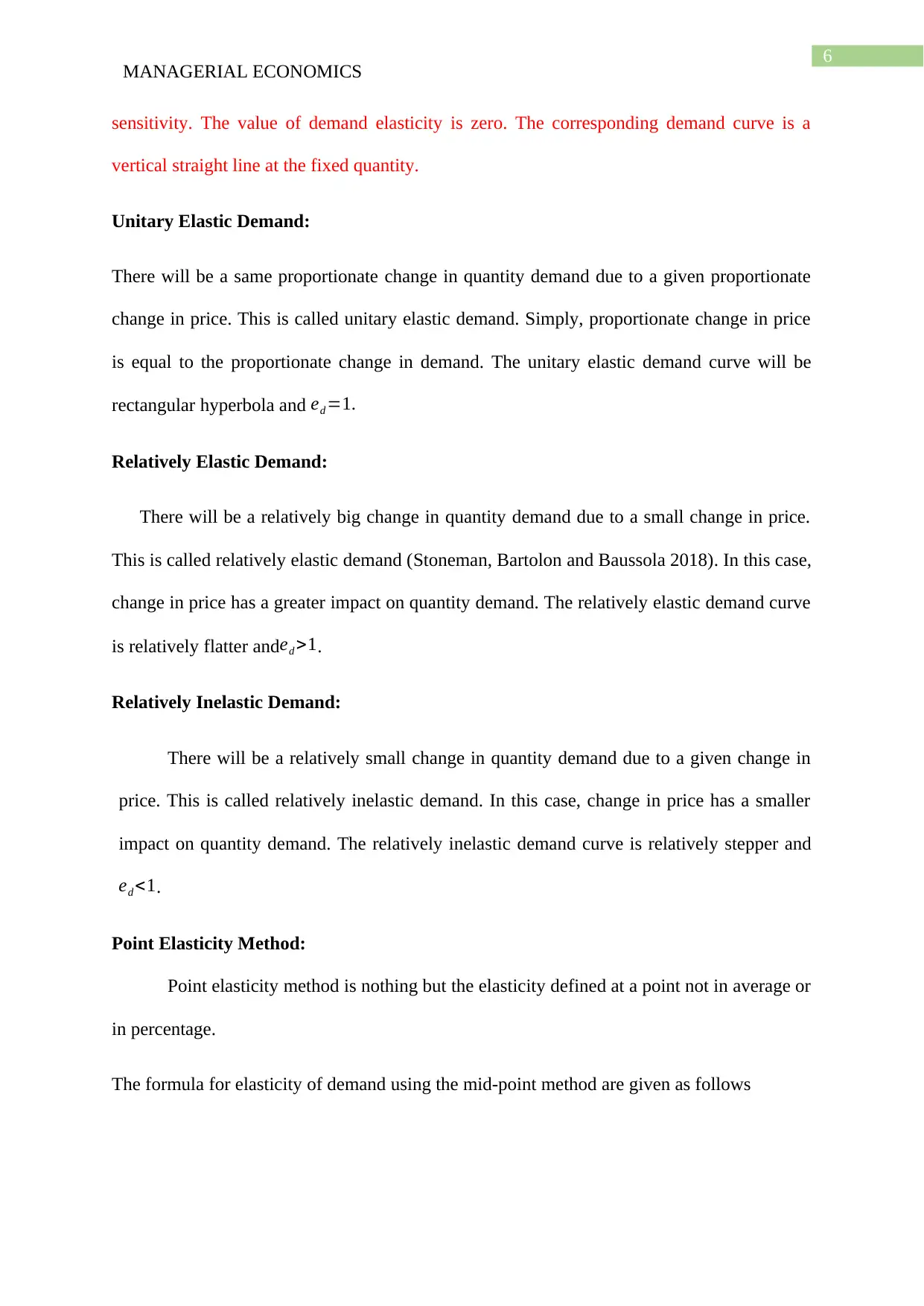
The formula for elasticity of demand using the mid-point method are given as follows

7
MANAGERIAL ECONOMICS
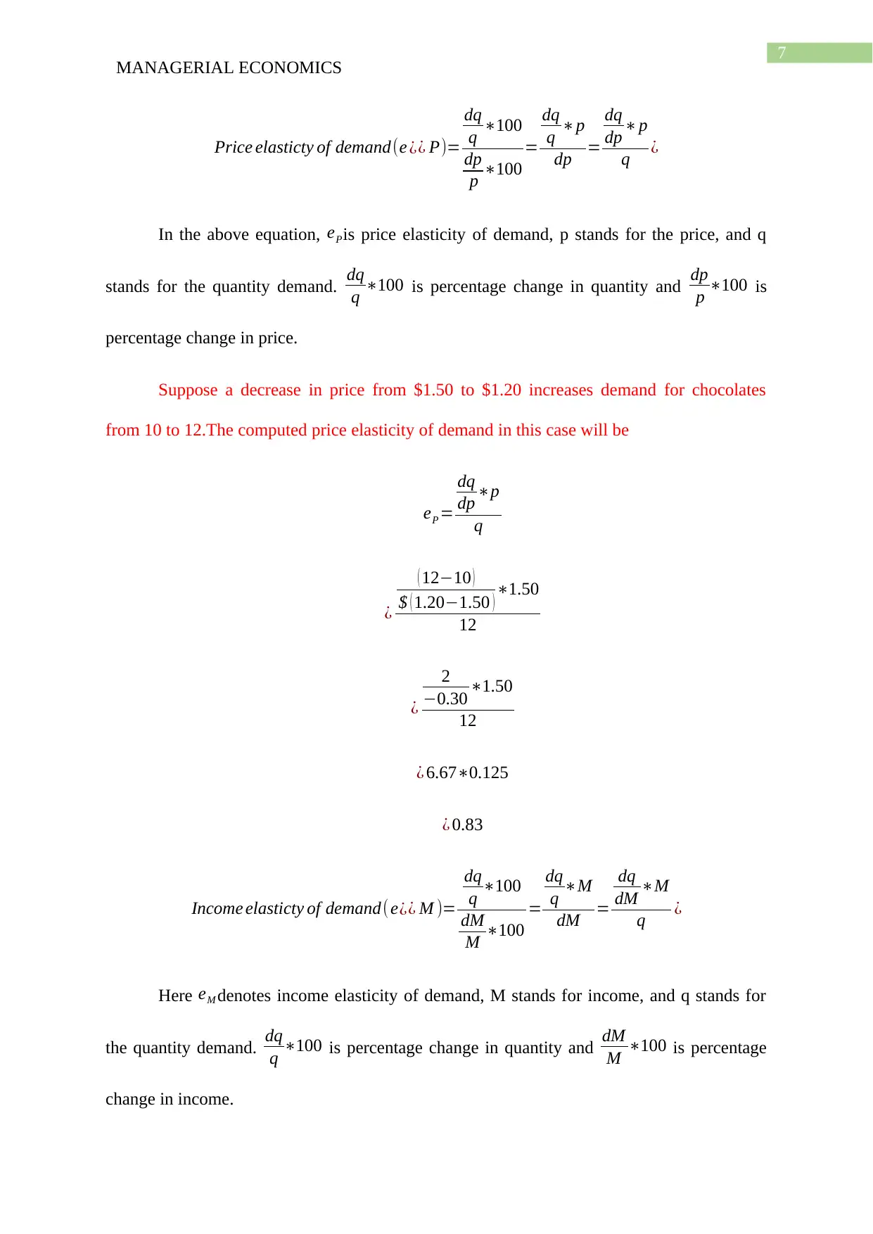
Price elasticty of demand(e ¿¿ P)=
dq
q ∗100
dp
p ∗100
=
dq
q ∗p
dp =
dq
dp ∗p
q ¿
In the above equation, ePis price elasticity of demand, p stands for the price, and q
stands for the quantity demand. dq
q ∗100 is percentage change in quantity and dp
p ∗100 is
percentage change in price.
Suppose a decrease in price from $1.50 to $1.20 increases demand for chocolates
from 10 to 12.The computed price elasticity of demand in this case will be
eP =
dq
dp ∗p
q
¿
( 12−10 )
$ ( 1.20−1.50 ) ∗1.50
12
¿
2
−0.30 ∗1.50
12
¿ 6.67∗0.125
¿ 0.83
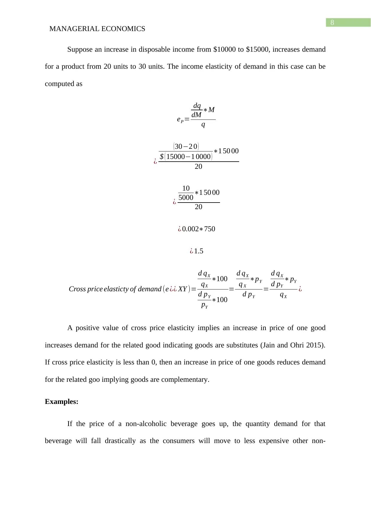
Income elasticty of demand( e¿¿ M )=
dq
q ∗100
dM
M ∗100
=
dq
q ∗M
dM =
dq
dM ∗M
q ¿
Here eM denotes income elasticity of demand, M stands for income, and q stands for
the quantity demand. dq
q ∗100 is percentage change in quantity and dM
M ∗100 is percentage
change in income.

8
MANAGERIAL ECONOMICS
Suppose an increase in disposable income from $10000 to $15000, increases demand
for a product from 20 units to 30 units. The income elasticity of demand in this case can be
computed as
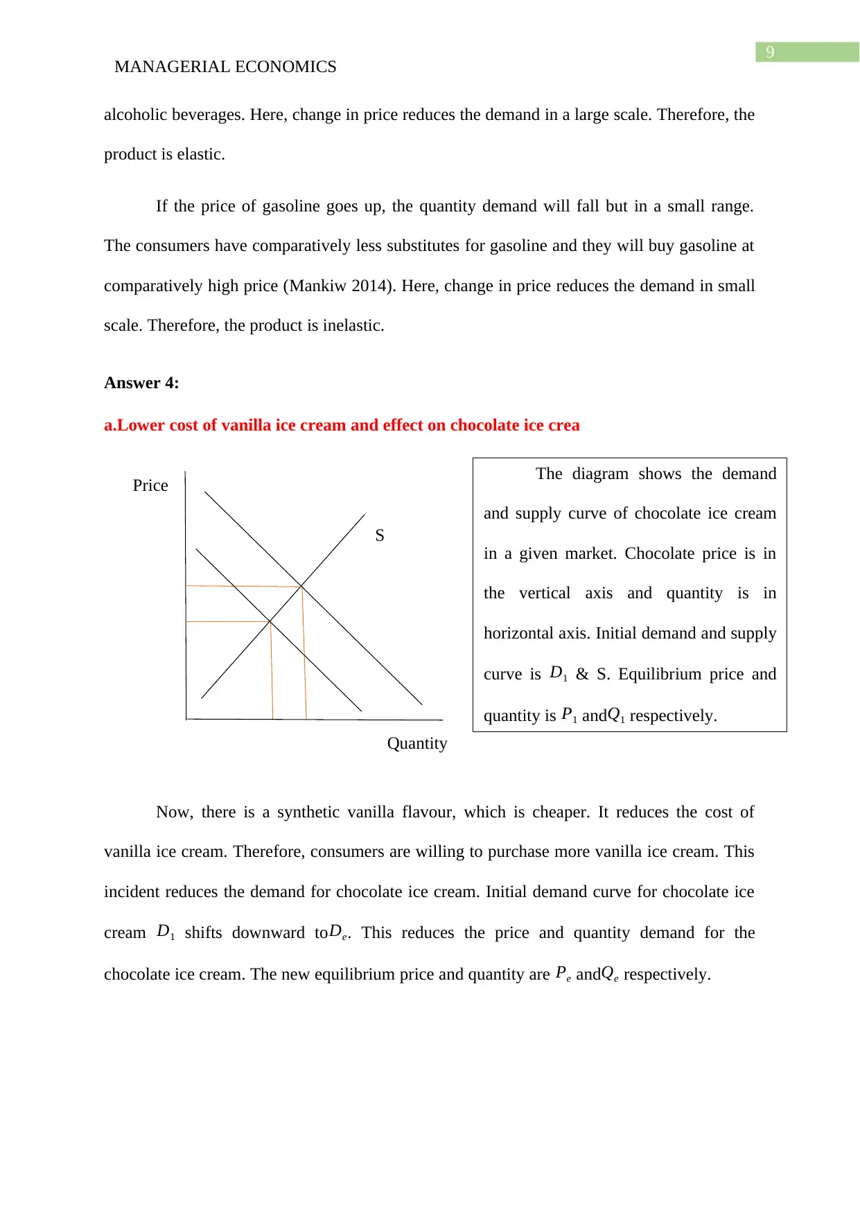
eP =
dq
dM ∗M
q
¿
(30−2 0 )
$ ( 15000−1 0000 ) ∗1 50 00
20
¿
10
5000∗1 50 00
20
¿ 0.002∗750
¿ 1.5
Cross price elasticty of demand (e ¿¿ XY )=
d qX
qX
∗100
d pY
pY
∗100
=
d qX
q X
∗pY
d pY
=
d qX
d pY
∗pY
qX
¿
A positive value of cross price elasticity implies an increase in price of one good
increases demand for the related good indicating goods are substitutes (Jain and Ohri 2015).
If cross price elasticity is less than 0, then an increase in price of one goods reduces demand
for the related goo implying goods are complementary.
Examples:
If the price of a non-alcoholic beverage goes up, the quantity demand for that
beverage will fall drastically as the consumers will move to less expensive other non-

9
MANAGERIAL ECONOMICS
Price
Quantity
S
alcoholic beverages. Here, change in price reduces the demand in a large scale. Therefore, the
product is elastic.
If the price of gasoline goes up, the quantity demand will fall but in a small range.
The consumers have comparatively less substitutes for gasoline and they will buy gasoline at
comparatively high price (Mankiw 2014). Here, change in price reduces the demand in small
scale. Therefore, the product is inelastic.
Answer 4:
a.Lower cost of vanilla ice cream and effect on chocolate ice crea
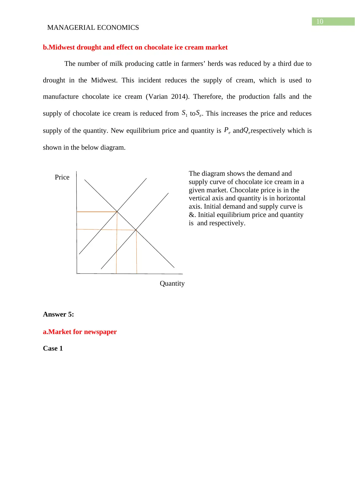
Now, there is a synthetic vanilla flavour, which is cheaper. It reduces the cost of
vanilla ice cream. Therefore, consumers are willing to purchase more vanilla ice cream. This
incident reduces the demand for chocolate ice cream. Initial demand curve for chocolate ice
cream D1 shifts downward toDe. This reduces the price and quantity demand for the
chocolate ice cream. The new equilibrium price and quantity are Pe andQe respectively.
The diagram shows the demand
and supply curve of chocolate ice cream
in a given market. Chocolate price is in
the vertical axis and quantity is in
horizontal axis. Initial demand and supply
curve is D1 & S. Equilibrium price and
quantity is P1 and Q1 respectively.

10
MANAGERIAL ECONOMICS
Price
Quantity
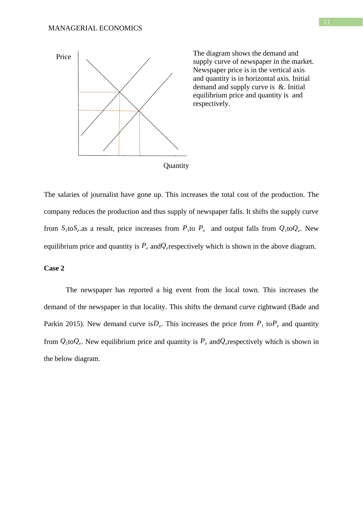
The diagram shows the demand and
supply curve of chocolate ice cream in a
given market. Chocolate price is in the
vertical axis and quantity is in horizontal
axis. Initial demand and supply curve is
&. Initial equilibrium price and quantity
is and respectively.
b.Midwest drought and effect on chocolate ice cream market
The number of milk producing cattle in farmers’ herds was reduced by a third due to
drought in the Midwest. This incident reduces the supply of cream, which is used to
manufacture chocolate ice cream (Varian 2014). Therefore, the production falls and the
supply of chocolate ice cream is reduced from S1 to Se. This increases the price and reduces
supply of the quantity. New equilibrium price and quantity is Pe andQerespectively which is
shown in the below diagram.
Answer 5:
a.Market for newspaper
Case 1

11
MANAGERIAL ECONOMICS
Price
Quantity
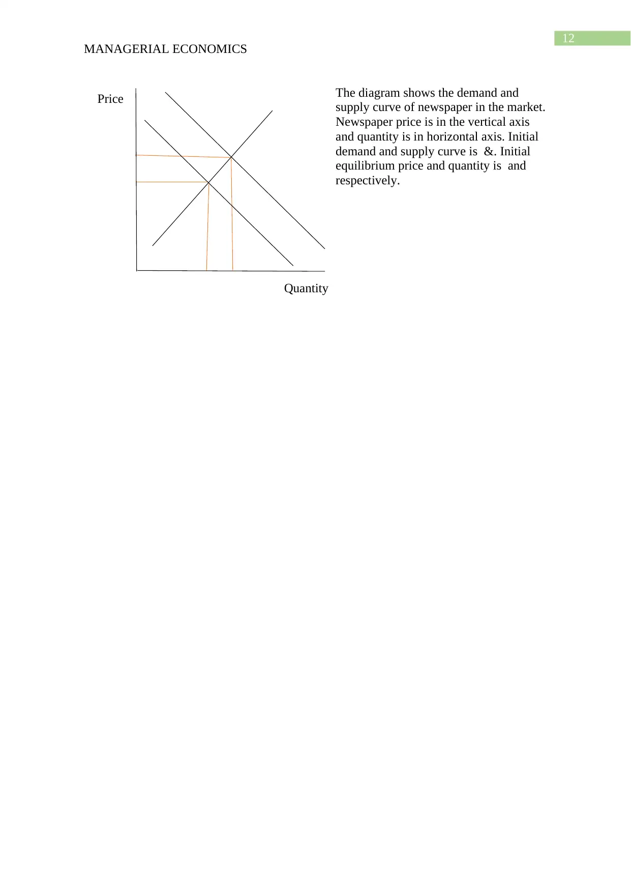
The diagram shows the demand and
supply curve of newspaper in the market.
Newspaper price is in the vertical axis
and quantity is in horizontal axis. Initial
demand and supply curve is &. Initial
equilibrium price and quantity is and
respectively.
The salaries of journalist have gone up. This increases the total cost of the production. The
company reduces the production and thus supply of newspaper falls. It shifts the supply curve
from S1toSe.as a result, price increases from P1to Pe and output falls from Q1toQe. New
equilibrium price and quantity is Pe andQerespectively which is shown in the above diagram.
Case 2
The newspaper has reported a big event from the local town. This increases the
demand of the newspaper in that locality. This shifts the demand curve rightward (Bade and
Parkin 2015). New demand curve isDe. This increases the price from P1 toPe and quantity
from Q1toQe. New equilibrium price and quantity is Pe and Qerespectively which is shown in
the below diagram.

12
MANAGERIAL ECONOMICS
Price
Quantity
The diagram shows the demand and
supply curve of newspaper in the market.
Newspaper price is in the vertical axis
and quantity is in horizontal axis. Initial
demand and supply curve is &. Initial
equilibrium price and quantity is and
respectively.

13
MANAGERIAL ECONOMICS
Price
Quantity
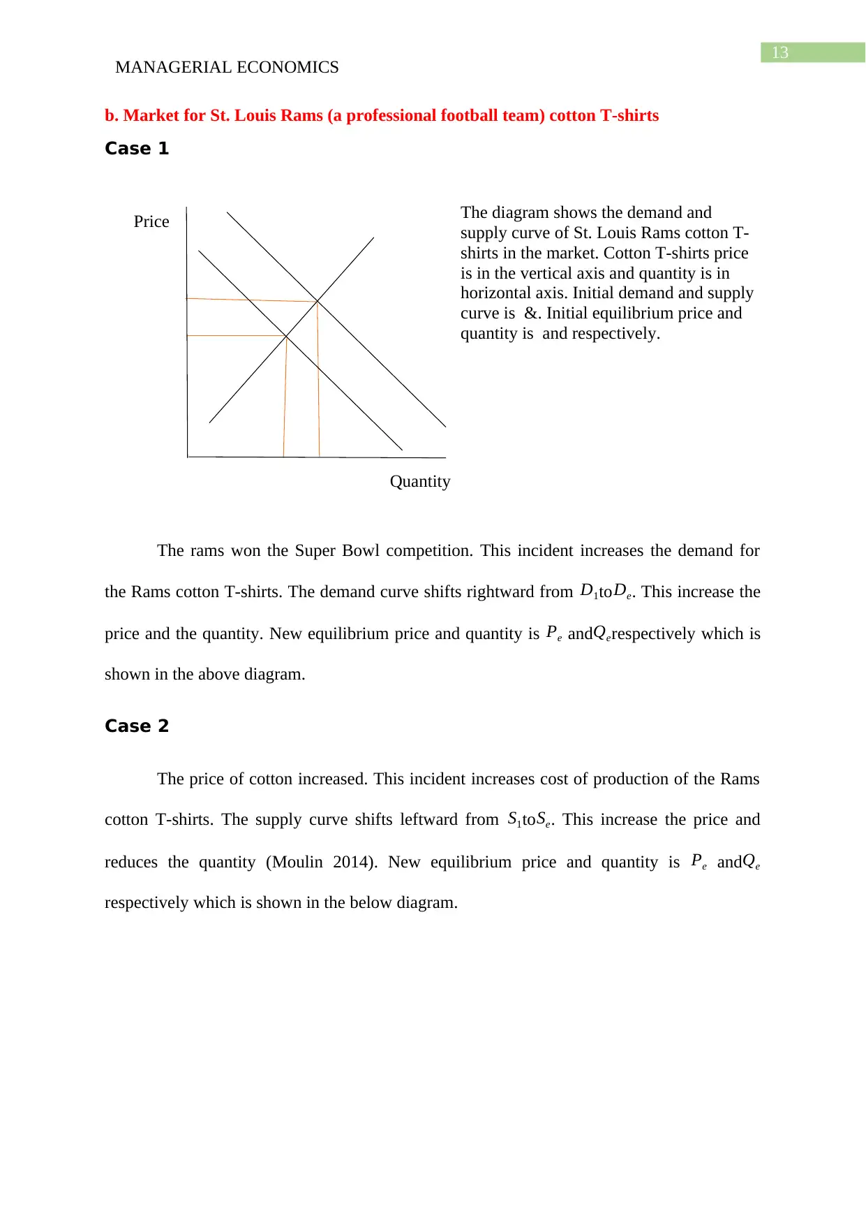
The diagram shows the demand and
supply curve of St. Louis Rams cotton T-
shirts in the market. Cotton T-shirts price
is in the vertical axis and quantity is in
horizontal axis. Initial demand and supply
curve is &. Initial equilibrium price and
quantity is and respectively.
b. Market for St. Louis Rams (a professional football team) cotton T-shirts
Case 1
The rams won the Super Bowl competition. This incident increases the demand for
the Rams cotton T-shirts. The demand curve shifts rightward from D1toDe. This increase the
price and the quantity. New equilibrium price and quantity is Pe and Qerespectively which is
shown in the above diagram.
Case 2
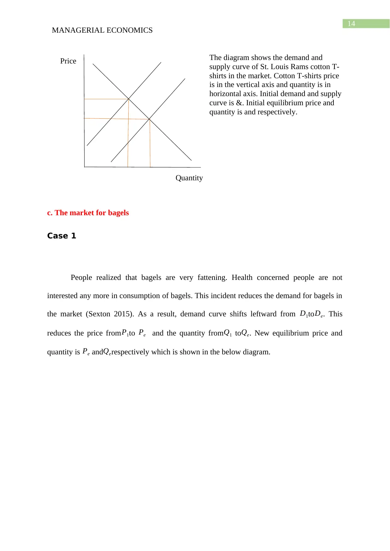
The price of cotton increased. This incident increases cost of production of the Rams
cotton T-shirts. The supply curve shifts leftward from S1toSe. This increase the price and
reduces the quantity (Moulin 2014). New equilibrium price and quantity is Pe and Qe
respectively which is shown in the below diagram.

14
MANAGERIAL ECONOMICS
Price
Quantity
The diagram shows the demand and
supply curve of St. Louis Rams cotton T-
shirts in the market. Cotton T-shirts price
is in the vertical axis and quantity is in
horizontal axis. Initial demand and supply
curve is &. Initial equilibrium price and
quantity is and respectively.
c. The market for bagels
Case 1
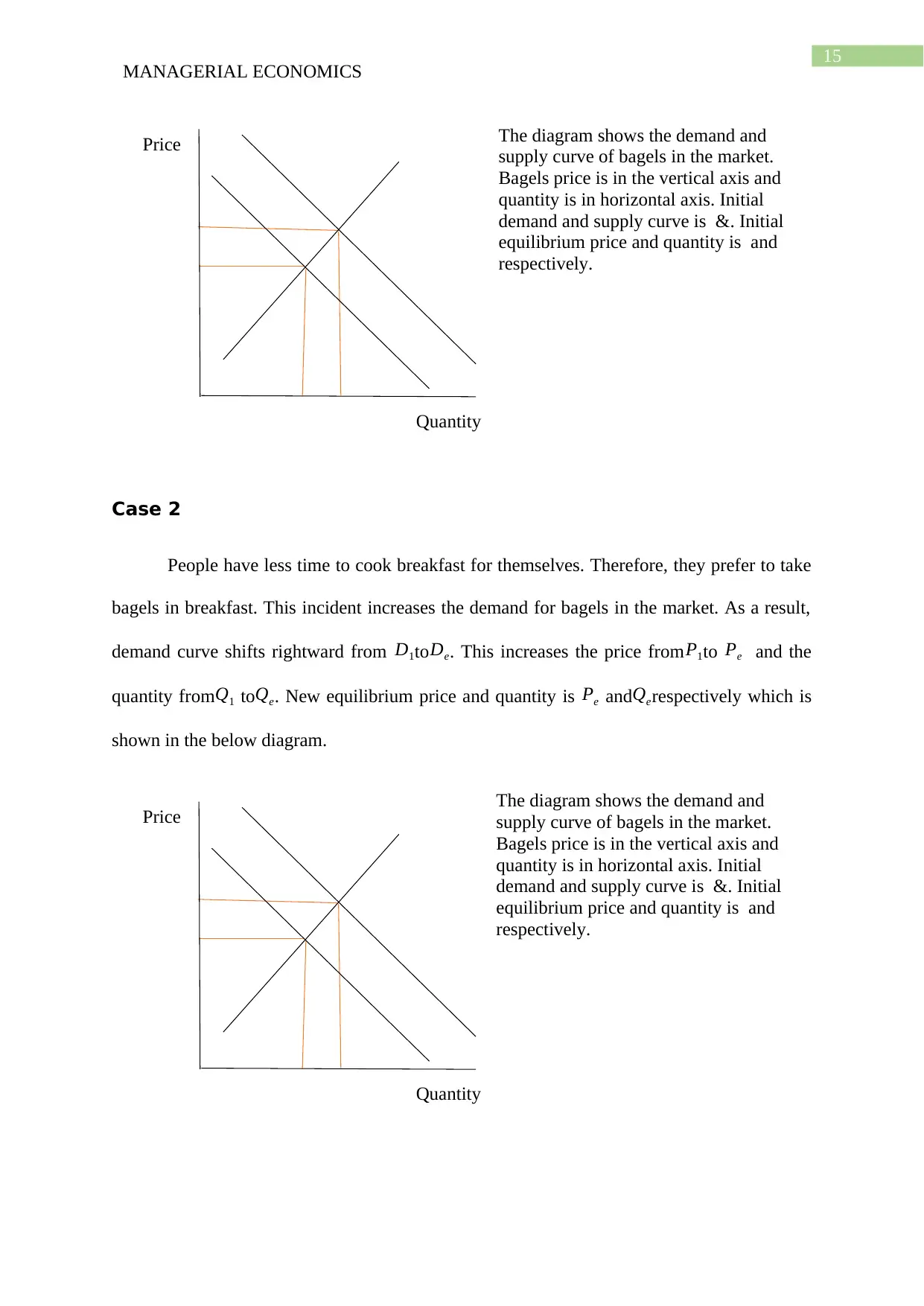
People realized that bagels are very fattening. Health concerned people are not
interested any more in consumption of bagels. This incident reduces the demand for bagels in
the market (Sexton 2015). As a result, demand curve shifts leftward from D1toDe. This
reduces the price from P1to Pe and the quantity from Q1 to Qe. New equilibrium price and
quantity is Pe andQerespectively which is shown in the below diagram.

15
MANAGERIAL ECONOMICS
Price
Quantity
The diagram shows the demand and
supply curve of bagels in the market.
Bagels price is in the vertical axis and
quantity is in horizontal axis. Initial
demand and supply curve is &. Initial
equilibrium price and quantity is and
respectively.
Price
Quantity
The diagram shows the demand and
supply curve of bagels in the market.
Bagels price is in the vertical axis and
quantity is in horizontal axis. Initial
demand and supply curve is &. Initial
equilibrium price and quantity is and
respectively.
Case 2
People have less time to cook breakfast for themselves. Therefore, they prefer to take
bagels in breakfast. This incident increases the demand for bagels in the market. As a result,
demand curve shifts rightward from D1to De. This increases the price from P1to Pe and the
quantity fromQ1 to Qe. New equilibrium price and quantity is Pe and Qerespectively which is
shown in the below diagram.

16
MANAGERIAL ECONOMICS
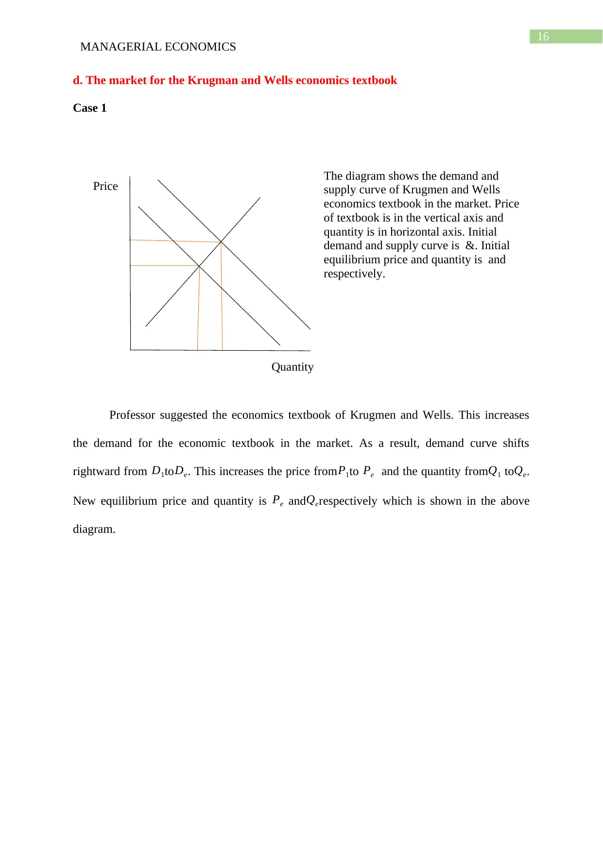
Price
Quantity
The diagram shows the demand and
supply curve of Krugmen and Wells
economics textbook in the market. Price
of textbook is in the vertical axis and
quantity is in horizontal axis. Initial
demand and supply curve is &. Initial
equilibrium price and quantity is and
respectively.
d. The market for the Krugman and Wells economics textbook
Case 1
Professor suggested the economics textbook of Krugmen and Wells. This increases
the demand for the economic textbook in the market. As a result, demand curve shifts
rightward from D1toDe. This increases the price fromP1to Pe and the quantity fromQ1 toQe.
New equilibrium price and quantity is Pe and Qerespectively which is shown in the above
diagram.

17
MANAGERIAL ECONOMICS
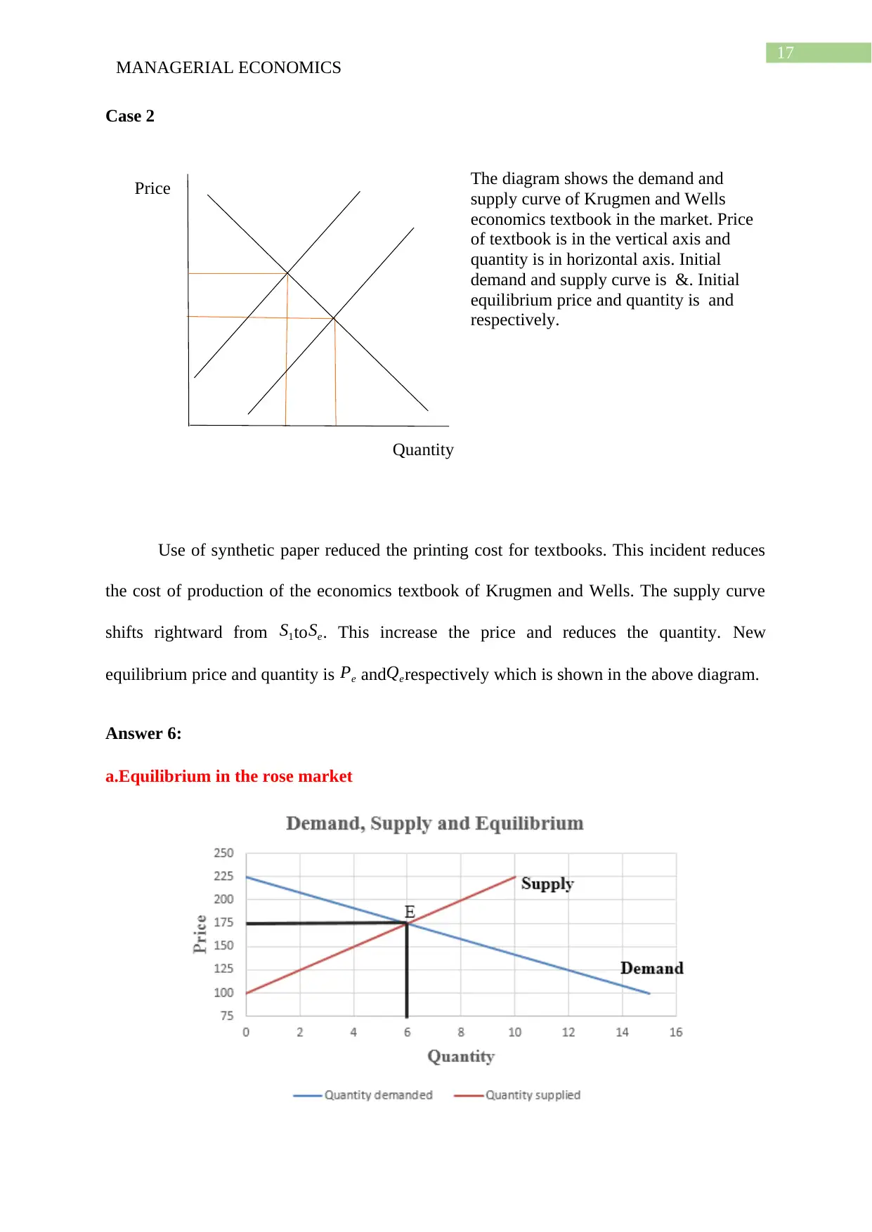
Price
Quantity
The diagram shows the demand and
supply curve of Krugmen and Wells
economics textbook in the market. Price
of textbook is in the vertical axis and
quantity is in horizontal axis. Initial
demand and supply curve is &. Initial
equilibrium price and quantity is and
respectively.
Case 2
Use of synthetic paper reduced the printing cost for textbooks. This incident reduces
the cost of production of the economics textbook of Krugmen and Wells. The supply curve
shifts rightward from S1toSe. This increase the price and reduces the quantity. New
equilibrium price and quantity is Pe andQerespectively which is shown in the above diagram.
Answer 6:
a.Equilibrium in the rose market

18
MANAGERIAL ECONOMICS
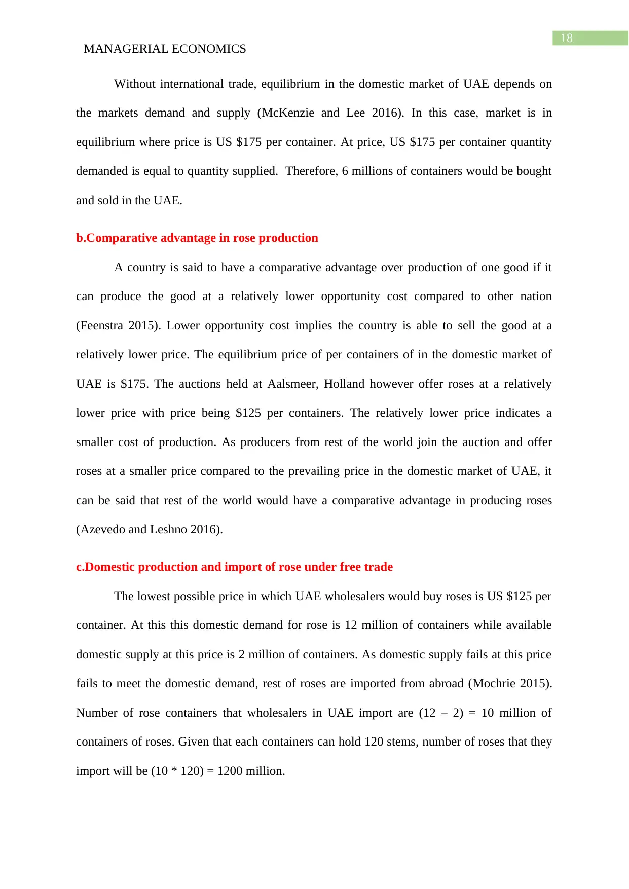
Without international trade, equilibrium in the domestic market of UAE depends on
the markets demand and supply (McKenzie and Lee 2016). In this case, market is in
equilibrium where price is US $175 per container. At price, US $175 per container quantity
demanded is equal to quantity supplied. Therefore, 6 millions of containers would be bought
and sold in the UAE.
b.Comparative advantage in rose production
A country is said to have a comparative advantage over production of one good if it
can produce the good at a relatively lower opportunity cost compared to other nation
(Feenstra 2015). Lower opportunity cost implies the country is able to sell the good at a
relatively lower price. The equilibrium price of per containers of in the domestic market of
UAE is $175. The auctions held at Aalsmeer, Holland however offer roses at a relatively
lower price with price being $125 per containers. The relatively lower price indicates a
smaller cost of production. As producers from rest of the world join the auction and offer
roses at a smaller price compared to the prevailing price in the domestic market of UAE, it
can be said that rest of the world would have a comparative advantage in producing roses
(Azevedo and Leshno 2016).
c.Domestic production and import of rose under free trade
The lowest possible price in which UAE wholesalers would buy roses is US $125 per
container. At this this domestic demand for rose is 12 million of containers while available
domestic supply at this price is 2 million of containers. As domestic supply fails at this price
fails to meet the domestic demand, rest of roses are imported from abroad (Mochrie 2015).
Number of rose containers that wholesalers in UAE import are (12 – 2) = 10 million of
containers of roses. Given that each containers can hold 120 stems, number of roses that they
import will be (10 * 120) = 1200 million.

19
MANAGERIAL ECONOMICS
Answer 7:
a.Market structure of telecommunication market
The market structure of telecommunication industry in UAE initially operated under a
framework of a monopoly market. Before, 2006 the market was a monopoly having a single
seller Etisalat in the industry. However, since 2006, the market became duopoly with two
players Etisalat and Du (Sharma 2014). Recently, a new telecom brand Virgin has started to
operate in the industry. Assuming the trend continues and government allows more
competitors (private and foreign players) in the market the market tends to become a
monopolistically competitive market (Boland 2017). In this form of market, there are
characteristics of competitive and monopoly market. Each telecommunication brand has a
monopoly power over its own brand. With increase in number of firms in the industry, there
would be intense competition among different brands in the industry. The main features of
emerging market structure in the telecommunication industry are, a relatively large size of
buyers and sellers, free entry or exit in the industry, high degree of product differentiation in
the form of different subscription plan, high spending on advertising, imperfect information
and a relatively high demand elasticity (Stiglitz et al. 2015).
b.Expected pricing strategies in the industry
In a monopolistically competitive market each brand uses its own pricing strategies
for own product or service. Three common pricing strategies used by most of the businesses
today are penetration pricing, skimming pricing and prestige pricing strategy (Arrow 2015).
Penetration refers to a pricing strategy in which a company introduces a low priced product in
order to capture a higher market share. Price skimming strategy refers to the strategy of profit
maximization by charging a relatively higher price to early adopters of the product and then
gradually reducing the price to attract the thriftier customers. A cell phone company for
example may launch new product initially with a high price taking advantage of people’s

20
MANAGERIAL ECONOMICS
willingness to pay a premium price for the innovative technology (Waldman and Jensen
2016). Once sales increased, the company then progressively reduces its price. Prestige
pricing strategy is a strategy of setting of setting price above the normal price as low price
hurts sales instead of boosting sales. Examples of goods having this kind of pricing strategy
include jewellery, high-end perfumes, cars, clothing and other luxury items. In the
telecommunication industry, the new firms are expected to use penetration-pricing strategy
(Belleflamme and Peitz 2015). Given the earlier duopoly structure of the market, the two
firms enjoyed significant market power. In order to attract customers, the new firms should
adapt penetration strategy.
Conclusion
From the discussion so far made suggests that main factors affecting supply of a good
are own price, technology, input price and cost of production. A change in demand or supply
condition leads to a change in equilibrium price and quantity. Finally, with change in number
of competitors, there is an associated change in market structure and pricing strategies of
firms.

21
MANAGERIAL ECONOMICS
References
Arrow, K., 2015. Microeconomics and operations research: Their interactions and
differences. Information Systems Frontiers, 17(1), pp.3-9.
Azevedo, E.M. and Leshno, J.D., 2016. A supply and demand framework for two-sided
matching markets. Journal of Political Economy, 124(5), pp.1235-1268.
Bade, R. and Parkin, M., 2015. Foundations of microeconomics. Pearson.
Belleflamme, P. and Peitz, M., 2015. Industrial organization: markets and strategies.
Cambridge University Press.
Blad, M.C. and Keiding, H., 2014. Microeconomics: Institutions, equilibrium and
optimality (Vol. 30). Elsevier.
Boland, L.A., 2017. Equilibrium Models in Economics: Purposes and Critical Limitations.
Oxford University Press.
Cowell, F., 2018. Microeconomics: principles and analysis. Oxford University Press.
Cowen, T. and Tabarrok, A., 2015. Modern principles of microeconomics. Macmillan
International Higher Education.
Feenstra, R.C., 2015. Advanced international trade: theory and evidence. Princeton
university press.
Jain, T.R. and Ohri, V.K., 2015. Principal of Microeconomics. FK Publications.
Kreps, D.M., 2019. Microeconomics for managers. Princeton University Press.
Mahanty, A.K., 2014. Intermediate microeconomics with applications. Academic Press.
Mankiw, N.G., 2014. Principles of economics. Cengage Learning.

22
MANAGERIAL ECONOMICS
McKenzie, R.B. and Lee, D.R., 2016. Microeconomics for MBAs: The economic way of
thinking for managers. Cambridge University Press.
Mochrie, R., 2015. Intermediate microeconomics. Macmillan International Higher Education.
Moulin, H., 2014. Cooperative microeconomics: a game-theoretic introduction (Vol. 313).
Princeton University Press.
Nicholson, W. and Snyder, C., 2014. Intermediate microeconomics and its application.
Nelson Education.
Sexton, R.L., 2015. Exploring Microeconomics. Nelson Education.
Sharma, R.B., 2014. Customers satisfaction in telecom sector in Saudi Arabia: An empirical
investigation. European Scientific Journal, ESJ, 10(13).
Stiglitz, J.E., Walsh, C.E., Gow, J. and Richmond, B., 2015. Introductory Microeconomics.
John Wiley and Sons Australia, Limited.
Stoneman, P., Bartoloni, E. and Baussola, M., 2018. The Microeconomics of Product
Innovation. Oxford University Press.
Thompson, G.E., 2016. Microeconomics: A Computational Approach: A Computational
Approach. Routledge.
Varian, H.R., 2014. Intermediate microeconomics with calculus: a modern approach. WW
Norton & Company.
Waldman, D. and Jensen, E., 2016. Industrial organization: theory and practice. Routledge.