BE274 Managerial Economics: Optimizing Activity Level and Profit Goals
VerifiedAdded on 2023/06/17
|6
|1508
|422
Report
AI Summary
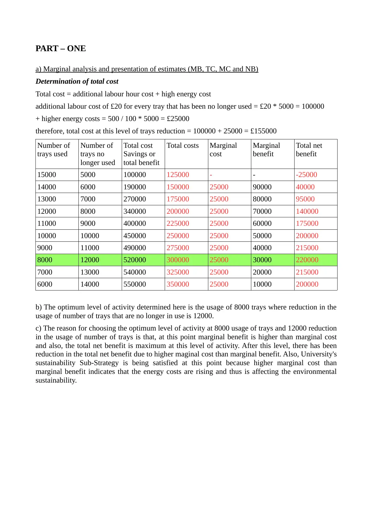
This report on Managerial Economics (BE274) provides an analysis of marginal benefits and costs to determine the optimum level of activity, focusing on tray usage reduction. It calculates total cost, marginal cost, and marginal benefit to identify the point where total net benefit is maximized. The report also discusses profit maximization as a primary goal of organizations, exploring reasons why firms may fail to achieve this objective, such as neglecting long-term sustainability, producing low-quality products, and inadequate employee training. Furthermore, it examines the relationship between profit maximization and social responsibility, arguing that social responsibility can contribute to long-term profitability by enhancing a company's image and reducing operational costs through sustainable practices. The report concludes that firms should balance profit maximization with ethical considerations and optimal resource utilization to contribute to both social welfare and economic success. Desklib offers a variety of study tools and resources for students.

1 out of 6
Your All-in-One AI-Powered Toolkit for Academic Success.
+13062052269
info@desklib.com
Available 24*7 on WhatsApp / Email
![[object Object]](/_next/static/media/star-bottom.7253800d.svg)
Copyright © 2020–2026 A2Z Services. All Rights Reserved. Developed and managed by ZUCOL.