Managerial Economics: Analyzing Market Forces and Elasticity
VerifiedAdded on 2023/04/25
|29
|5345
|61
Report
AI Summary
This report provides a comprehensive analysis of managerial economics principles, focusing on supply, demand, and elasticity. It begins by defining the supply schedule and exploring factors affecting supply, such as commodity price, prices of other goods, input costs, technology, and government policies. The report then discusses the concept of perfectly inelastic demand and its impact on market equilibrium, demonstrating how increased supply affects equilibrium price when demand remains constant. Further, it delves into the degrees of elasticity of demand, including perfectly elastic, perfectly inelastic, unitary elastic, elastic, and inelastic demand, supported by relevant diagrams. The point elasticity method is also explained, along with examples of goods with elastic and inelastic demand. Finally, the report applies these concepts to analyze specific market scenarios, such as the market for newspapers, St. Louis Rams T-shirts, bagels, and economics textbooks, providing a thorough understanding of market dynamics and elasticity in various contexts.
Running head: MANAGERIAL ECONOMICS
Managerial Economics
Name of the Student
Name of the University
Student ID
Managerial Economics
Name of the Student
Name of the University
Student ID
Paraphrase This Document
Need a fresh take? Get an instant paraphrase of this document with our AI Paraphraser
1MANAGERIAL ECONOMICS
Table of Contents
Question 1..................................................................................................................................3
Question a...............................................................................................................................3
Question b..............................................................................................................................5
Question 2..................................................................................................................................6
Degrees of elasticity of demand.............................................................................................6
Point elasticity method.........................................................................................................11
Question 3................................................................................................................................13
Question a.............................................................................................................................13
Question b............................................................................................................................14
Question 4................................................................................................................................16
Question a.............................................................................................................................16
Question b............................................................................................................................17
Question 5................................................................................................................................18
Question a: market for newspaper in the town.....................................................................18
Question b: The market for St. Louis Rams cotton T-shirts................................................20
Question c: The market for bagels.......................................................................................21
Question d: The market for Krugman and Wells economics textbook................................23
Question 6................................................................................................................................24
Question a.............................................................................................................................24
Question b............................................................................................................................25
Question c.............................................................................................................................25
References................................................................................................................................26
2MANAGERIAL ECONOMICS
Question 1
Question a
Supply schedule
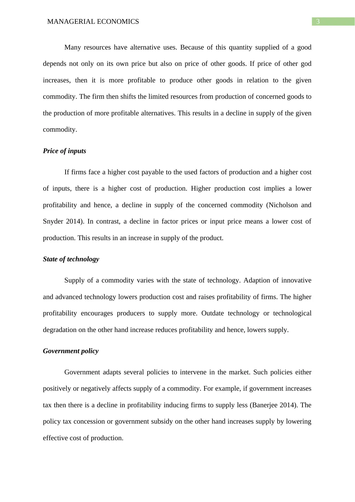
Supply schedule is the presentation of quantity supplied corresponding to various
prices in a table form. The supply schedule shows various quantities of the supplied good at
different prices. It indicates relation between price and quantity supplied when all other non-
price factors remain constant. Supply schedules are of two kinds. These are individual supply
schedule and market supply schedule (Varian 2014). The individual supply schedule captures
the supply of an individual seller or firm in relation to own price. In contrast, market supply
schedule is the sum of individual supply schedules. It represents total supply in the market at
various prices.
Different factors affecting supply
In the market, there are different important factors that determine supply of a good.
Change in any of these factors lead to a corresponding change in supply of the good. Given
below are some of the important factors affecting supply of a commodity.
Price of the commodity
The most vital determinant of supply is the price. Following the law of supply, there
is a direct relation between price and supply of a good. That means with increase in price of a
good its supply increases and vice versa. This is because of the simple reason. As price of
good increases, producers have a higher possibility of making profit (Wetzstein 2013). It
encourages them to supply more in order to increase sale in the market.
Price of other goods
Question 1
Question a
Supply schedule
Supply schedule is the presentation of quantity supplied corresponding to various
prices in a table form. The supply schedule shows various quantities of the supplied good at
different prices. It indicates relation between price and quantity supplied when all other non-
price factors remain constant. Supply schedules are of two kinds. These are individual supply
schedule and market supply schedule (Varian 2014). The individual supply schedule captures
the supply of an individual seller or firm in relation to own price. In contrast, market supply
schedule is the sum of individual supply schedules. It represents total supply in the market at
various prices.
Different factors affecting supply
In the market, there are different important factors that determine supply of a good.
Change in any of these factors lead to a corresponding change in supply of the good. Given
below are some of the important factors affecting supply of a commodity.
Price of the commodity
The most vital determinant of supply is the price. Following the law of supply, there
is a direct relation between price and supply of a good. That means with increase in price of a
good its supply increases and vice versa. This is because of the simple reason. As price of
good increases, producers have a higher possibility of making profit (Wetzstein 2013). It
encourages them to supply more in order to increase sale in the market.
Price of other goods
⊘ This is a preview!⊘
Do you want full access?
Subscribe today to unlock all pages.
Trusted by 1+ million students worldwide
3MANAGERIAL ECONOMICS
Many resources have alternative uses. Because of this quantity supplied of a good
depends not only on its own price but also on price of other goods. If price of other god
increases, then it is more profitable to produce other goods in relation to the given
commodity. The firm then shifts the limited resources from production of concerned goods to
the production of more profitable alternatives. This results in a decline in supply of the given
commodity.
Price of inputs
If firms face a higher cost payable to the used factors of production and a higher cost
of inputs, there is a higher cost of production. Higher production cost implies a lower
profitability and hence, a decline in supply of the concerned commodity (Nicholson and
Snyder 2014). In contrast, a decline in factor prices or input price means a lower cost of
production. This results in an increase in supply of the product.
State of technology
Supply of a commodity varies with the state of technology. Adaption of innovative
and advanced technology lowers production cost and raises profitability of firms. The higher
profitability encourages producers to supply more. Outdate technology or technological
degradation on the other hand increase reduces profitability and hence, lowers supply.
Government policy
Government adapts several policies to intervene in the market. Such policies either
positively or negatively affects supply of a commodity. For example, if government increases
tax then there is a decline in profitability inducing firms to supply less (Banerjee 2014). The
policy tax concession or government subsidy on the other hand increases supply by lowering
effective cost of production.
Paraphrase This Document
Need a fresh take? Get an instant paraphrase of this document with our AI Paraphraser
4MANAGERIAL ECONOMICS
Objective of the firm
As stated by law of supply, supply of a commodity increases at a higher price as a
relatively higher price fulfills firms’ profit maximization goal. Some firms however might
agree to supply more at a lower price even if the price does not maximize profits. The goals
of such firms is to capture a higher share in the market in order to strengthen their position in
the market.
Question b
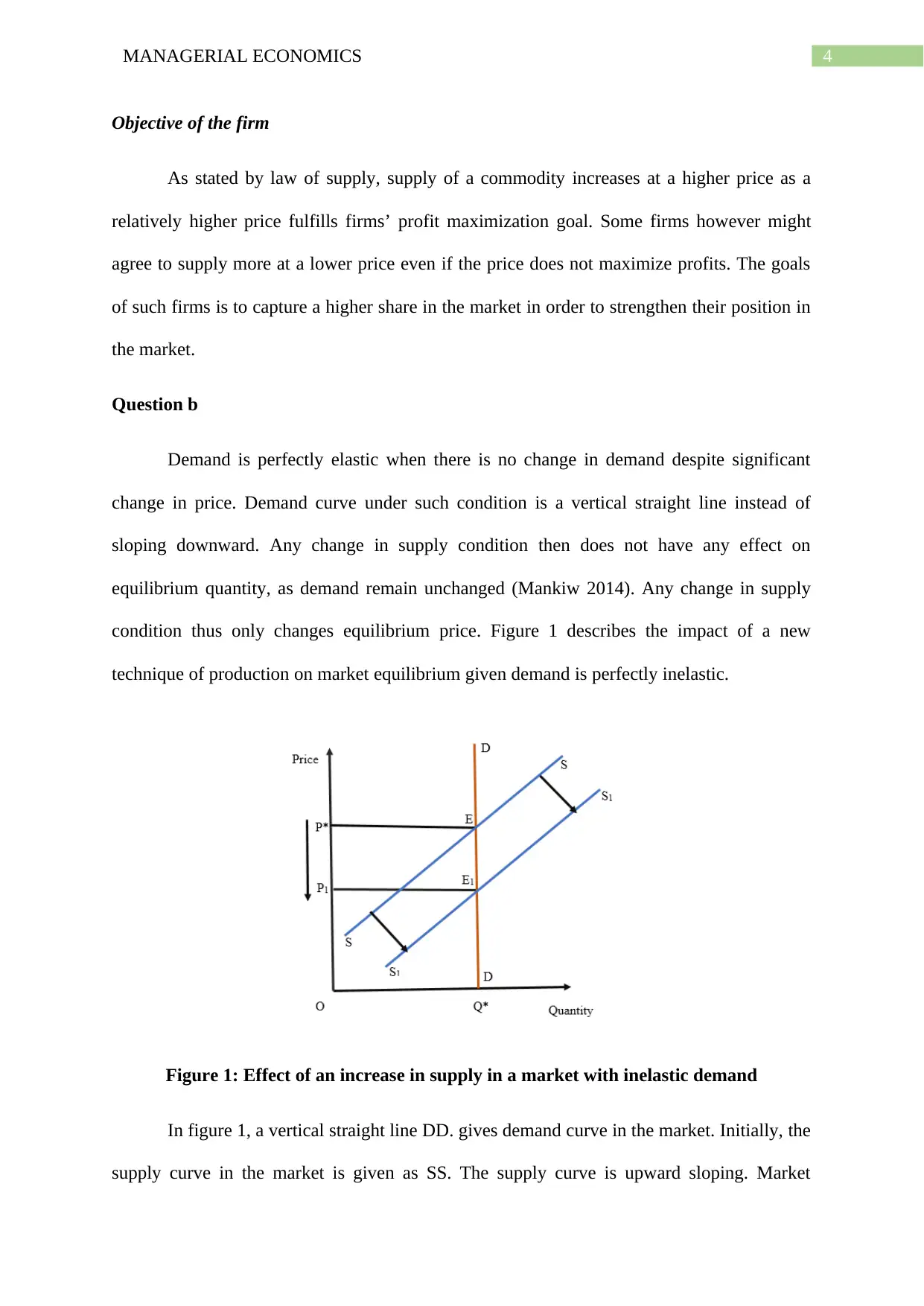
Demand is perfectly elastic when there is no change in demand despite significant
change in price. Demand curve under such condition is a vertical straight line instead of
sloping downward. Any change in supply condition then does not have any effect on
equilibrium quantity, as demand remain unchanged (Mankiw 2014). Any change in supply
condition thus only changes equilibrium price. Figure 1 describes the impact of a new
technique of production on market equilibrium given demand is perfectly inelastic.
Figure 1: Effect of an increase in supply in a market with inelastic demand
In figure 1, a vertical straight line DD. gives demand curve in the market. Initially, the
supply curve in the market is given as SS. The supply curve is upward sloping. Market
Objective of the firm
As stated by law of supply, supply of a commodity increases at a higher price as a
relatively higher price fulfills firms’ profit maximization goal. Some firms however might
agree to supply more at a lower price even if the price does not maximize profits. The goals
of such firms is to capture a higher share in the market in order to strengthen their position in
the market.
Question b
Demand is perfectly elastic when there is no change in demand despite significant
change in price. Demand curve under such condition is a vertical straight line instead of
sloping downward. Any change in supply condition then does not have any effect on
equilibrium quantity, as demand remain unchanged (Mankiw 2014). Any change in supply
condition thus only changes equilibrium price. Figure 1 describes the impact of a new
technique of production on market equilibrium given demand is perfectly inelastic.
Figure 1: Effect of an increase in supply in a market with inelastic demand
In figure 1, a vertical straight line DD. gives demand curve in the market. Initially, the
supply curve in the market is given as SS. The supply curve is upward sloping. Market
5MANAGERIAL ECONOMICS
equilibrium at the initial stance occurs at E. Corresponding to the equilibrium point,
equilibrium price is P* and equilibrium quantity is Q*. When application of innovative
technology doubles market supply, then market supply curve shifts to the right. New supply
curve in the market is given as S1S1. The new equilibrium in the market occurs where existing
demand curve intersects the new supply curve (Mahanty 2014). The new equilibrium point in
the above figure is obtained at E1. At the new equilibrium point, quantity in the market
remains same as Q*. The excess supply situation pushes market equilibrium price downward
to P1.
As reflected from the above figure, an increase in supply given perfectly inelastic
demand reduces market price keeping equilibrium quantity unchanged. As a result, producers
now experience a lower revenue. Increasing supply with perfectly inelastic demand therefore
is not beneficial for producers as it lowers revenue compared to earlier situation.
Question 2
Degrees of elasticity of demand
Price elasticity of demand refers to the proportionate change in demand following
certain proportionate change in price. Demand of a good is sensitive or responsive to a
change in price. Demand however does not vary uniformly following a price change (Cowell
2018). In some cases, a small change in demand causes a relatively large change in price
while in others relatively large price change causes quantity demand to change only by a
smaller extent.
Elastic and inelastic demand
An elastic demand refers to a situation where proportionate change in demand is
larger than the corresponding proportionate change in price. For example, suppose a decrease
in price by 1 percent leads to an increase in quantity demanded by 5%. In this case, demand
⊘ This is a preview!⊘
Do you want full access?
Subscribe today to unlock all pages.
Trusted by 1+ million students worldwide
6MANAGERIAL ECONOMICS
is considered as elastic demand. In contrast, there are products for which demand not very
much sensitive. For example, if a 5% increase in price causes demand to change by only 1%,
then demand is considered as inelastic (Labandeira, Labeaga and Lopez-Otero 2017).
The terms like elastic and inelastic do not completely capture the extent of responsiveness or
unresponsiveness of a quantity demanded of a product with respect to a change in price.
The degree of elasticity can be broadly categorized into five groups.
Perfectly elastic demand
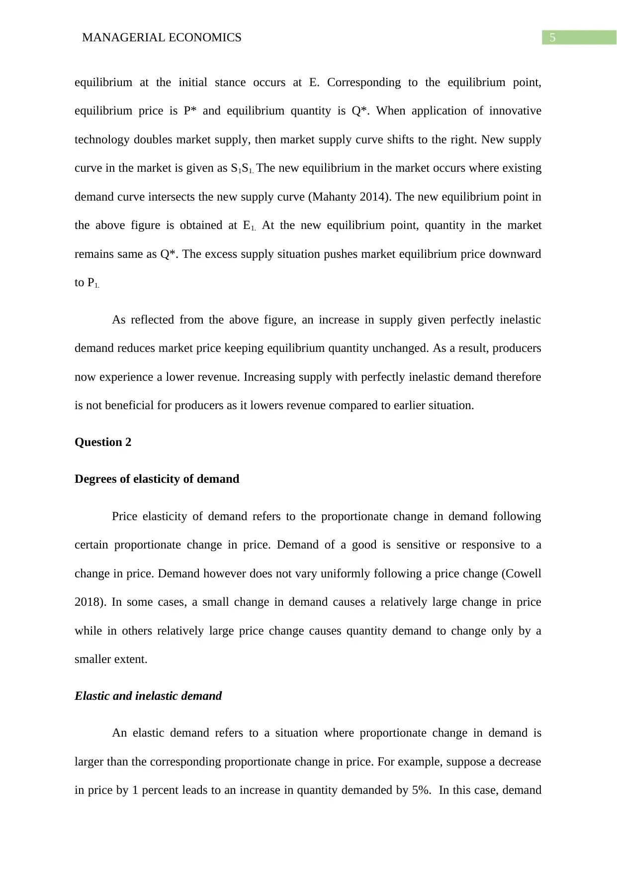
Demand is considered as perfectly elastic a small or no change in price results in large
change in infinite change in price. Perfectly elastic demand implies that sellers can sell
whatever quantity they want at a ruling price. They however cannot increase price in the
market (Imbs and Mejean 2015). If producers try to charge even one more unit of price, then
no one will buy the product. A perfectly elastic demand curve is given in the following
figure.
Figure 2: Perfectly elastic demand curve
is considered as elastic demand. In contrast, there are products for which demand not very
much sensitive. For example, if a 5% increase in price causes demand to change by only 1%,
then demand is considered as inelastic (Labandeira, Labeaga and Lopez-Otero 2017).
The terms like elastic and inelastic do not completely capture the extent of responsiveness or
unresponsiveness of a quantity demanded of a product with respect to a change in price.
The degree of elasticity can be broadly categorized into five groups.
Perfectly elastic demand
Demand is considered as perfectly elastic a small or no change in price results in large
change in infinite change in price. Perfectly elastic demand implies that sellers can sell
whatever quantity they want at a ruling price. They however cannot increase price in the
market (Imbs and Mejean 2015). If producers try to charge even one more unit of price, then
no one will buy the product. A perfectly elastic demand curve is given in the following
figure.
Figure 2: Perfectly elastic demand curve
Paraphrase This Document
Need a fresh take? Get an instant paraphrase of this document with our AI Paraphraser
7MANAGERIAL ECONOMICS
The above figure shows that the demand curve DD’ is a horizontal straight line
indicating that quantity demanded is highly responsiveness to change in price. The demand
curve DD’ is infinitely inelastic. The value of elasticity of demand in this case equals to
infinity.
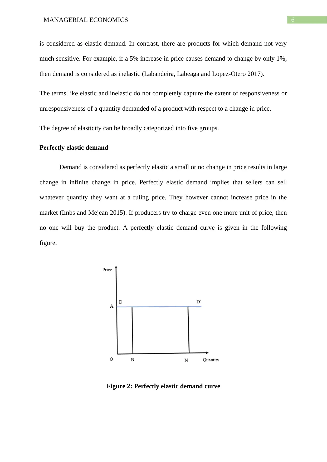
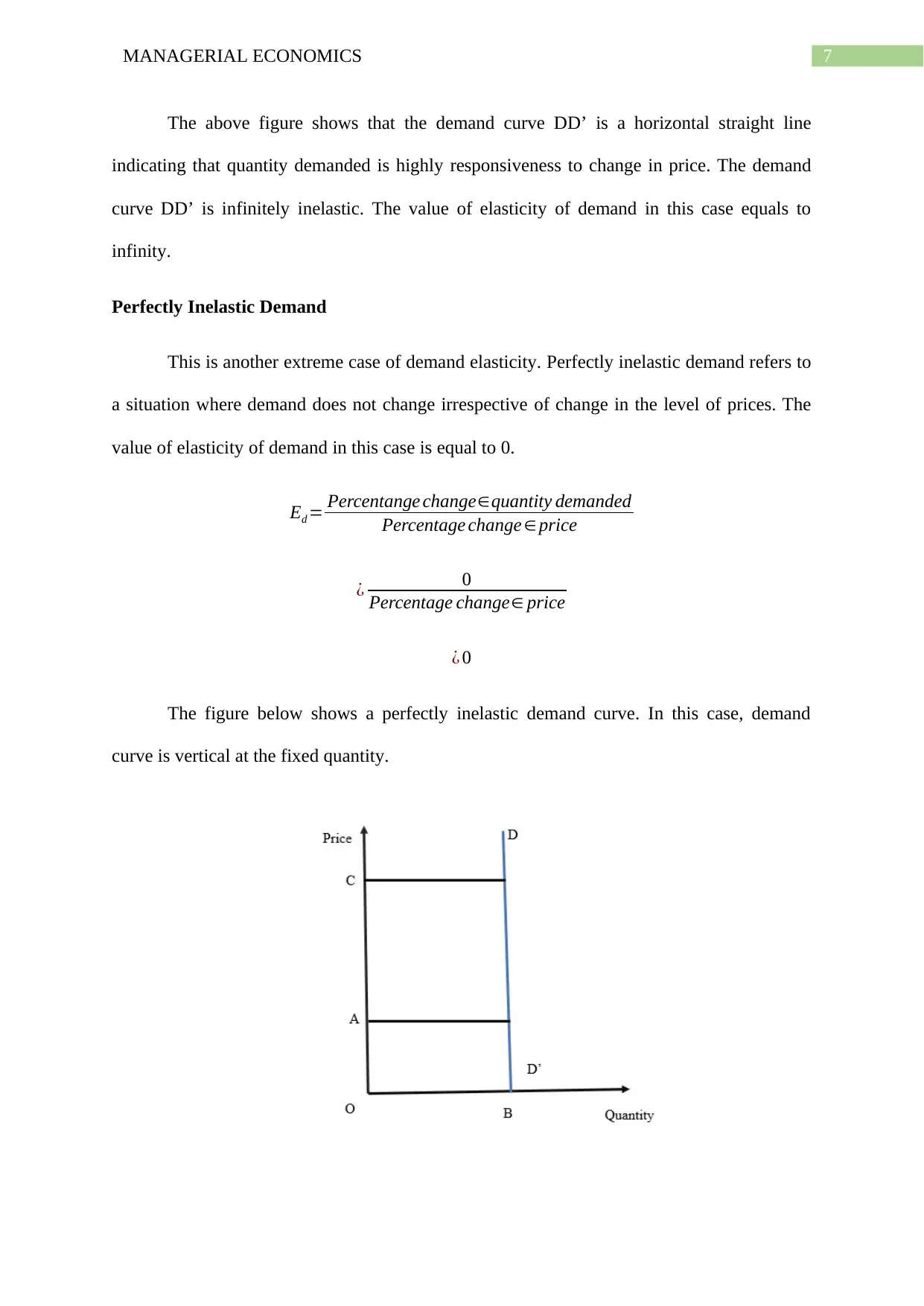
Perfectly Inelastic Demand
This is another extreme case of demand elasticity. Perfectly inelastic demand refers to
a situation where demand does not change irrespective of change in the level of prices. The
value of elasticity of demand in this case is equal to 0.
Ed = Percentange change∈quantity demanded
Percentage change ∈ price
¿ 0
Percentage change∈ price
¿ 0
The figure below shows a perfectly inelastic demand curve. In this case, demand
curve is vertical at the fixed quantity.
The above figure shows that the demand curve DD’ is a horizontal straight line
indicating that quantity demanded is highly responsiveness to change in price. The demand
curve DD’ is infinitely inelastic. The value of elasticity of demand in this case equals to
infinity.
Perfectly Inelastic Demand
This is another extreme case of demand elasticity. Perfectly inelastic demand refers to
a situation where demand does not change irrespective of change in the level of prices. The
value of elasticity of demand in this case is equal to 0.
Ed = Percentange change∈quantity demanded
Percentage change ∈ price
¿ 0
Percentage change∈ price
¿ 0
The figure below shows a perfectly inelastic demand curve. In this case, demand
curve is vertical at the fixed quantity.
8MANAGERIAL ECONOMICS
Figure 3: Perfectly inelastic demand
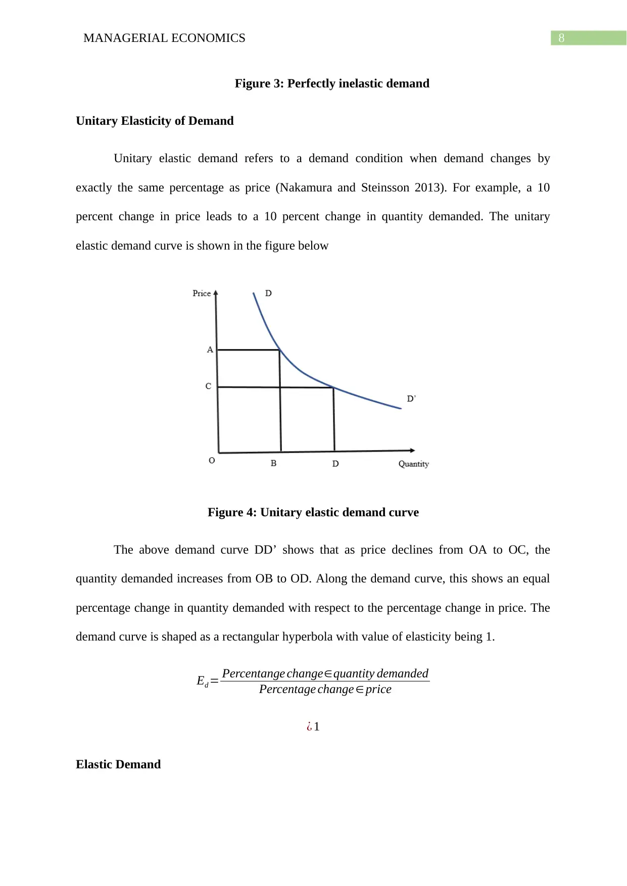
Unitary Elasticity of Demand
Unitary elastic demand refers to a demand condition when demand changes by
exactly the same percentage as price (Nakamura and Steinsson 2013). For example, a 10
percent change in price leads to a 10 percent change in quantity demanded. The unitary
elastic demand curve is shown in the figure below
Figure 4: Unitary elastic demand curve
The above demand curve DD’ shows that as price declines from OA to OC, the
quantity demanded increases from OB to OD. Along the demand curve, this shows an equal
percentage change in quantity demanded with respect to the percentage change in price. The
demand curve is shaped as a rectangular hyperbola with value of elasticity being 1.
Ed = Percentange change∈quantity demanded
Percentage change ∈ price
¿ 1
Elastic Demand
Figure 3: Perfectly inelastic demand
Unitary Elasticity of Demand
Unitary elastic demand refers to a demand condition when demand changes by
exactly the same percentage as price (Nakamura and Steinsson 2013). For example, a 10
percent change in price leads to a 10 percent change in quantity demanded. The unitary
elastic demand curve is shown in the figure below
Figure 4: Unitary elastic demand curve
The above demand curve DD’ shows that as price declines from OA to OC, the
quantity demanded increases from OB to OD. Along the demand curve, this shows an equal
percentage change in quantity demanded with respect to the percentage change in price. The
demand curve is shaped as a rectangular hyperbola with value of elasticity being 1.
Ed = Percentange change∈quantity demanded
Percentage change ∈ price
¿ 1
Elastic Demand
⊘ This is a preview!⊘
Do you want full access?
Subscribe today to unlock all pages.
Trusted by 1+ million students worldwide
9MANAGERIAL ECONOMICS
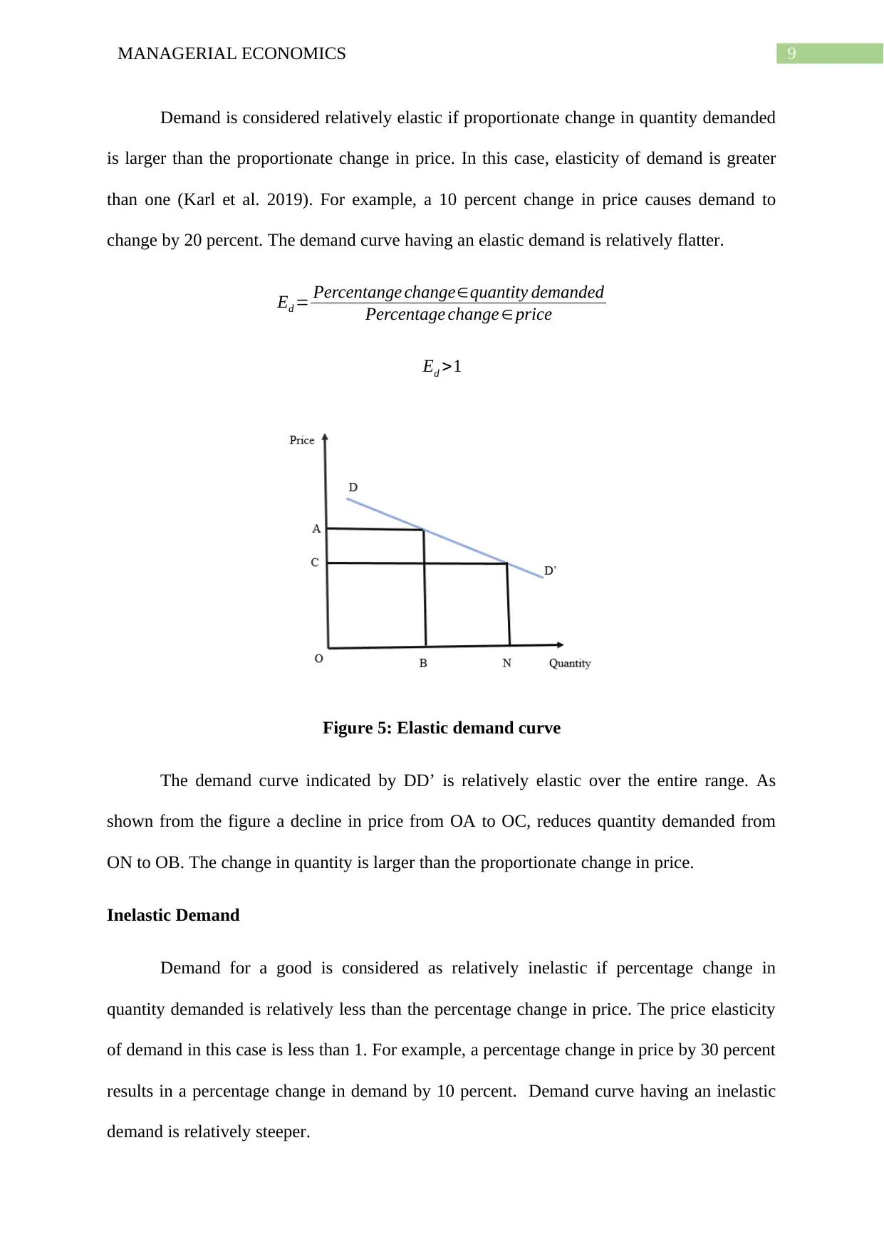
Demand is considered relatively elastic if proportionate change in quantity demanded
is larger than the proportionate change in price. In this case, elasticity of demand is greater
than one (Karl et al. 2019). For example, a 10 percent change in price causes demand to
change by 20 percent. The demand curve having an elastic demand is relatively flatter.
Ed = Percentange change∈quantity demanded
Percentage change ∈ price
Ed >1
Figure 5: Elastic demand curve
The demand curve indicated by DD’ is relatively elastic over the entire range. As
shown from the figure a decline in price from OA to OC, reduces quantity demanded from
ON to OB. The change in quantity is larger than the proportionate change in price.
Inelastic Demand
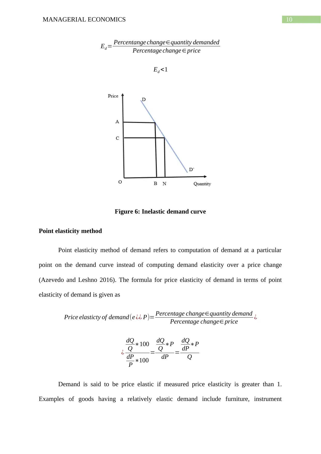
Demand for a good is considered as relatively inelastic if percentage change in
quantity demanded is relatively less than the percentage change in price. The price elasticity
of demand in this case is less than 1. For example, a percentage change in price by 30 percent
results in a percentage change in demand by 10 percent. Demand curve having an inelastic
demand is relatively steeper.
Demand is considered relatively elastic if proportionate change in quantity demanded
is larger than the proportionate change in price. In this case, elasticity of demand is greater
than one (Karl et al. 2019). For example, a 10 percent change in price causes demand to
change by 20 percent. The demand curve having an elastic demand is relatively flatter.
Ed = Percentange change∈quantity demanded
Percentage change ∈ price
Ed >1
Figure 5: Elastic demand curve
The demand curve indicated by DD’ is relatively elastic over the entire range. As
shown from the figure a decline in price from OA to OC, reduces quantity demanded from
ON to OB. The change in quantity is larger than the proportionate change in price.
Inelastic Demand
Demand for a good is considered as relatively inelastic if percentage change in
quantity demanded is relatively less than the percentage change in price. The price elasticity
of demand in this case is less than 1. For example, a percentage change in price by 30 percent
results in a percentage change in demand by 10 percent. Demand curve having an inelastic
demand is relatively steeper.
Paraphrase This Document
Need a fresh take? Get an instant paraphrase of this document with our AI Paraphraser
10MANAGERIAL ECONOMICS
Ed = Percentange change∈quantity demanded
Percentage change ∈ price
Ed <1
Figure 6: Inelastic demand curve
Point elasticity method
Point elasticity method of demand refers to computation of demand at a particular
point on the demand curve instead of computing demand elasticity over a price change
(Azevedo and Leshno 2016). The formula for price elasticity of demand in terms of point
elasticity of demand is given as
Price elasticty of demand(e ¿¿ P)= Percentage change∈quantity demand
Percentage change∈ price ¿
¿
dQ
Q ∗100
dP
P ∗100
=
dQ
Q ∗P
dP =
dQ
dP ∗P
Q
Demand is said to be price elastic if measured price elasticity is greater than 1.
Examples of goods having a relatively elastic demand include furniture, instrument
11MANAGERIAL ECONOMICS
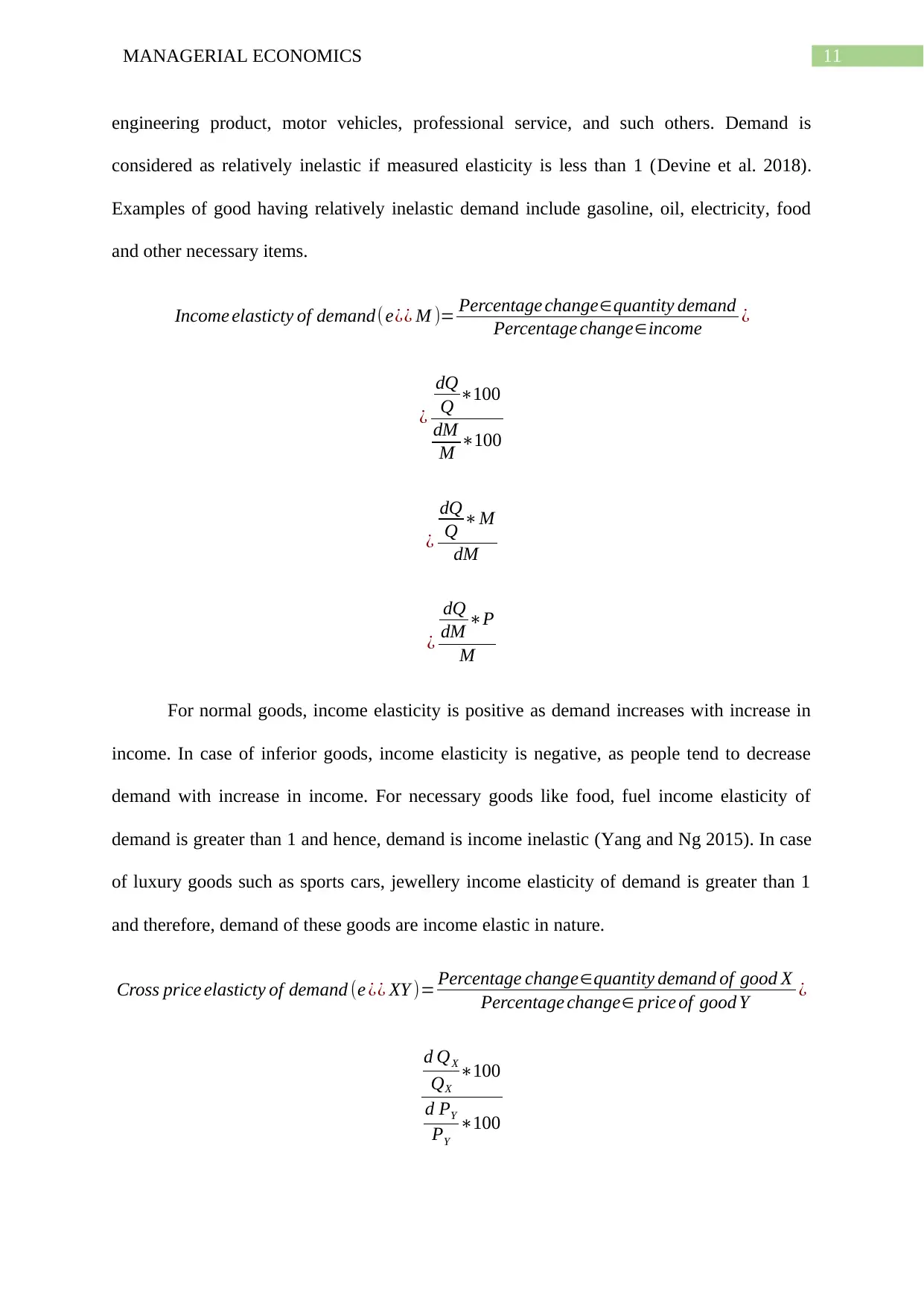
engineering product, motor vehicles, professional service, and such others. Demand is
considered as relatively inelastic if measured elasticity is less than 1 (Devine et al. 2018).
Examples of good having relatively inelastic demand include gasoline, oil, electricity, food
and other necessary items.
Income elasticty of demand( e¿¿ M )= Percentage change∈quantity demand
Percentage change∈income ¿
¿
dQ
Q ∗100
dM
M ∗100
¿
dQ
Q ∗M
dM
¿
dQ
dM ∗P
M
For normal goods, income elasticity is positive as demand increases with increase in
income. In case of inferior goods, income elasticity is negative, as people tend to decrease
demand with increase in income. For necessary goods like food, fuel income elasticity of
demand is greater than 1 and hence, demand is income inelastic (Yang and Ng 2015). In case
of luxury goods such as sports cars, jewellery income elasticity of demand is greater than 1
and therefore, demand of these goods are income elastic in nature.
Cross price elasticty of demand (e ¿¿ XY )= Percentage change∈quantity demand of good X
Percentage change∈ price of good Y ¿
d QX
QX
∗100
d PY
PY
∗100
⊘ This is a preview!⊘
Do you want full access?
Subscribe today to unlock all pages.
Trusted by 1+ million students worldwide
1 out of 29
Related Documents


Your All-in-One AI-Powered Toolkit for Academic Success.
+13062052269
info@desklib.com
Available 24*7 on WhatsApp / Email
![[object Object]](/_next/static/media/star-bottom.7253800d.svg)
Unlock your academic potential
Copyright © 2020–2026 A2Z Services. All Rights Reserved. Developed and managed by ZUCOL.