Managing Data

Managing data indicates the interpretation and analysis of the data that has been collected using statistical and other tools. The current report will use different statistical concepts and obtain results based on the different requirements of the questions.

MANAGING DATA

TABLE OF CONTENTS
INTRODUCTION...........................................................................................................................3
QUESTIONS...................................................................................................................................3
QUESTION 1..................................................................................................................................3
a. Three main sources..................................................................................................................3
b. Calculation...............................................................................................................................3
c. Best chart.................................................................................................................................5
d. Is primary data qualitative data................................................................................................5
QUESTION 2..................................................................................................................................6
a. Probability of spending over £10.............................................................................................6
b. Frequency of over 1 mile.........................................................................................................6
c. Modal group.............................................................................................................................6
d. Simple Interest.........................................................................................................................7
e. Compound Interest...................................................................................................................7
QUESTION 3..................................................................................................................................8
a. Marks to be achieved...............................................................................................................8
b. Test Score for 95% interval.....................................................................................................8
c. Probability................................................................................................................................8
QUESTION 4................................................................................................................................10
a. Statistical relationship............................................................................................................10
b. Values of Parameters.............................................................................................................10
c. Recommendations..................................................................................................................12
CONCLUSION..............................................................................................................................12
EXCEL..........................................................................................................................................13
QUESTION 1................................................................................................................................13
QUESTION 4................................................................................................................................14

INTRODUCTION
Managing data indicates the interpretation and analysis of the data that has been collected
using statistical and other tools (Druschke and et.al., 2020). The current report will use different
statistical concepts and obtain results based on the different requirements of the questions.
QUESTIONS
QUESTION 1
a. Three main sources
Primary data is the data that is collected on a first hand basis by the researcher i.e. this
data has not been collected or used prior to this research and is original (Johnston, 2017). The
primary data for the research can be collected using sources such as Personal Interview,
Questionnaire Method, and Case Study Analysis etc.
Secondary data is the one that has already been published and is used in the existing
research because it holds some points of relevance in the present study being conducted
(Fishman and Chai, OpenTV Inc, 2019). The sources of secondary data are previously published
research papers and journals, Government or Company Reports, Encyclopedias etc.
b. Calculation
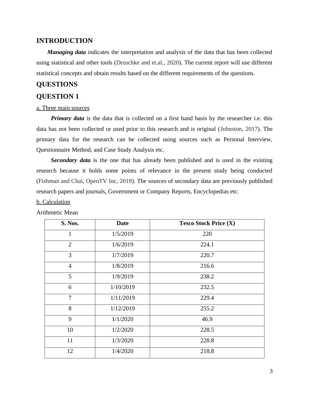
Arithmetic Mean
S. Nos. Date Tesco Stock Price (X)
1 1/5/2019 220
2 1/6/2019 224.1
3 1/7/2019 220.7
4 1/8/2019 216.6
5 1/9/2019 238.2
6 1/10/2019 232.5
7 1/11/2019 229.4
8 1/12/2019 255.2
9 1/1/2020 46.9
10 1/2/2020 228.5
11 1/3/2020 228.8
12 1/4/2020 218.8
3

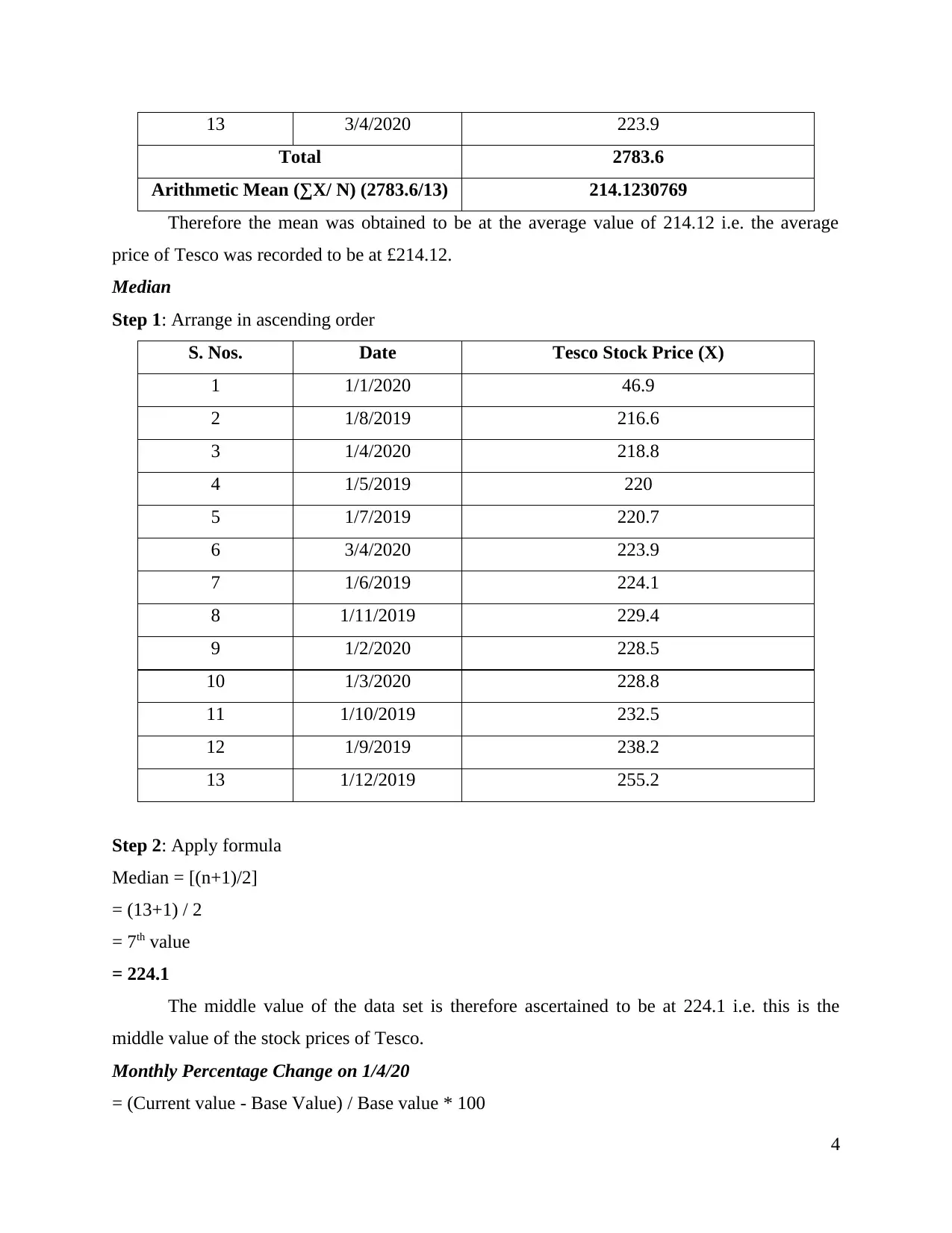
13 3/4/2020 223.9
Total 2783.6
Arithmetic Mean (∑X/ N) (2783.6/13) 214.1230769
Therefore the mean was obtained to be at the average value of 214.12 i.e. the average
price of Tesco was recorded to be at £214.12.
Median
Step 1: Arrange in ascending order
S. Nos. Date Tesco Stock Price (X)
1 1/1/2020 46.9
2 1/8/2019 216.6
3 1/4/2020 218.8
4 1/5/2019 220
5 1/7/2019 220.7
6 3/4/2020 223.9
7 1/6/2019 224.1
8 1/11/2019 229.4
9 1/2/2020 228.5
10 1/3/2020 228.8
11 1/10/2019 232.5
12 1/9/2019 238.2
13 1/12/2019 255.2
Step 2: Apply formula
Median = [(n+1)/2]
= (13+1) / 2
= 7th value
= 224.1
The middle value of the data set is therefore ascertained to be at 224.1 i.e. this is the
middle value of the stock prices of Tesco.
Monthly Percentage Change on 1/4/20
= (Current value - Base Value) / Base value * 100
4

= (218.8 - 228.8) / 228.8 * 100
= -4%
This therefore shows a negative movement i.e. decline of the stock prices of Tesco by a 4%
change in one month period as on 1/04/20.
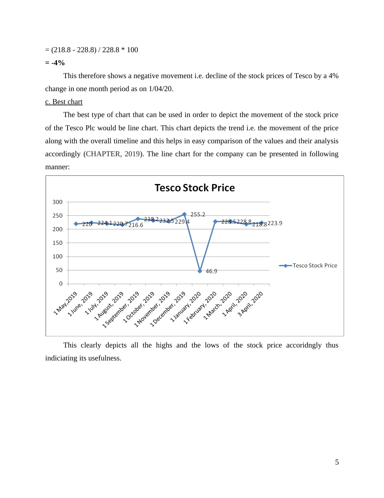
c. Best chart
The best type of chart that can be used in order to depict the movement of the stock price
of the Tesco Plc would be line chart. This chart depicts the trend i.e. the movement of the price
along with the overall timeline and this helps in easy comparison of the values and their analysis
accordingly (CHAPTER, 2019). The line chart for the company can be presented in following
manner:
This clearly depicts all the highs and the lows of the stock price accoridngly thus
indiciating its usefulness.
5

d. Is primary data qualitative data
The statement made by Abbi is wrong as the primary data can be both qualitative data and
quantitative data based on the nature of the research data that has been collected. For instance,
qualitative primary data can be in the form of observation method, interview method, case study
analysis etc. and the quantitative primary data can be collected through questionnaire method,
surveys etc. (Arrieta, Souza and Calili, 2018). Therefore it would be wrong to state that primary
data is only qualitative data.
QUESTION 2
a. Probability of spending over £10
The basic formula for calculation of probability can be ascertained as:
P (E) = Number of favourable outcomes/ Total number of outcomes
Where, P (E) denotes the probability of an event E.
Now here, probability has to be ascertained for the event that Mike incurs a travel expense over £
10.
The number of students who incur expense over £ 10 are 19 and the total number of
students travelling over a distance of one mile are 10 + 20 + 19 i.e. 49.
Therefore the probability of this event can be calculated in following manner:
P (E) = 19 / 49
P (E) = 0.39
Therefore there are 0.39 chances that mike might incur an expense above the £ 10 while
travelling to his campus.
b. Frequency of over 1 mile
Frequency is basically the total number of successful events of something happening over
the total number of events (Wang, 2019). In context of probability, this is also classified as
relative frequency where the frequency of the likely chance of an event to occur is ascertained.
In the current scenario, the frequency of the students living more than 1 mile away from the
campus needs to be calculated and the successful students can be obtained as 10 + 20 + 19 i.e.
49. Now the total number of students being studied in the sample is 185. Therefore, the relative
frequency is:
RF = Number of successful trials / total number of trials
6

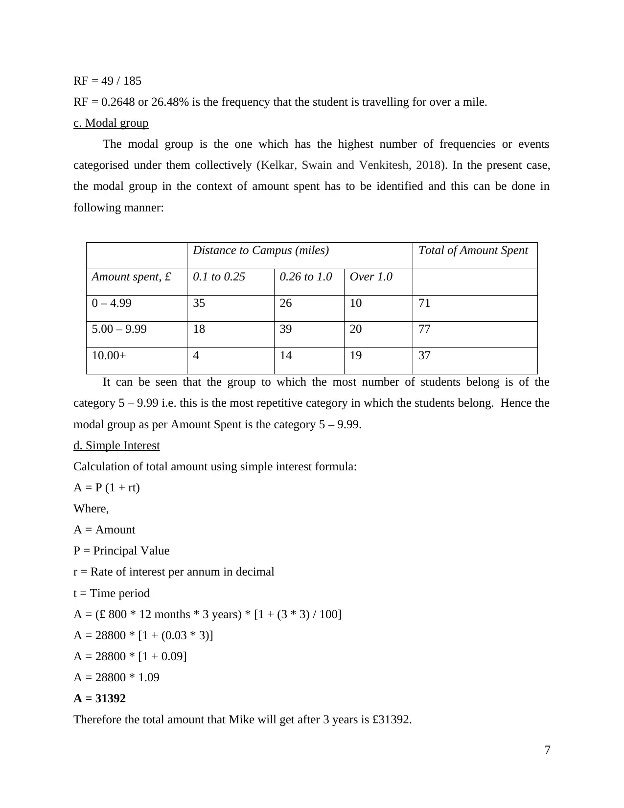
RF = 49 / 185
RF = 0.2648 or 26.48% is the frequency that the student is travelling for over a mile.
c. Modal group
The modal group is the one which has the highest number of frequencies or events
categorised under them collectively (Kelkar, Swain and Venkitesh, 2018). In the present case,
the modal group in the context of amount spent has to be identified and this can be done in
following manner:
Distance to Campus (miles) Total of Amount Spent
Amount spent, £ 0.1 to 0.25 0.26 to 1.0 Over 1.0
0 – 4.99 35 26 10 71
5.00 – 9.99 18 39 20 77
10.00+ 4 14 19 37
It can be seen that the group to which the most number of students belong is of the
category 5 – 9.99 i.e. this is the most repetitive category in which the students belong. Hence the
modal group as per Amount Spent is the category 5 – 9.99.
d. Simple Interest
Calculation of total amount using simple interest formula:
A = P (1 + rt)
Where,
A = Amount
P = Principal Value
r = Rate of interest per annum in decimal
t = Time period
A = (£ 800 * 12 months * 3 years) * [1 + (3 * 3) / 100]
A = 28800 * [1 + (0.03 * 3)]
A = 28800 * [1 + 0.09]
A = 28800 * 1.09
A = 31392
Therefore the total amount that Mike will get after 3 years is £31392.
7

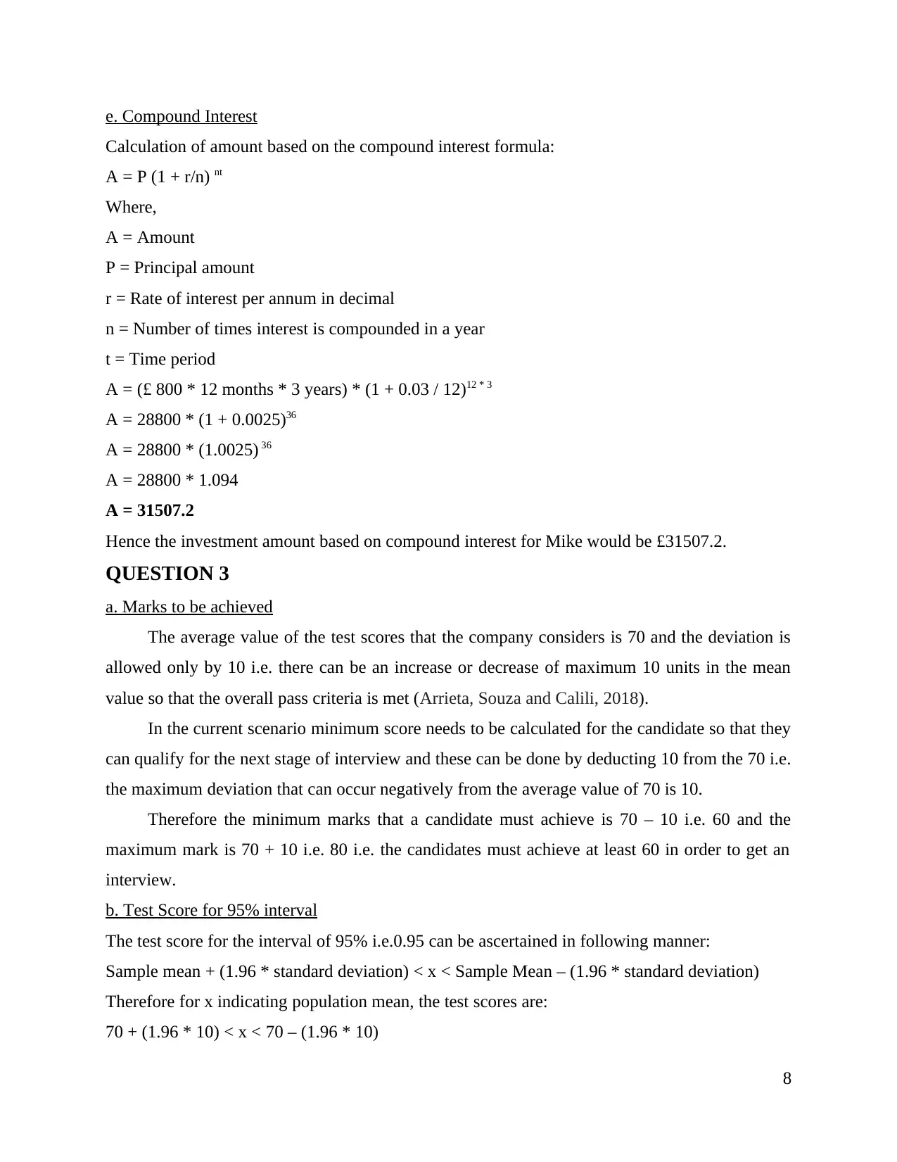
e. Compound Interest
Calculation of amount based on the compound interest formula:
A = P (1 + r/n) nt
Where,
A = Amount
P = Principal amount
r = Rate of interest per annum in decimal
n = Number of times interest is compounded in a year
t = Time period
A = (£ 800 * 12 months * 3 years) * (1 + 0.03 / 12)12 * 3
A = 28800 * (1 + 0.0025)36
A = 28800 * (1.0025) 36
A = 28800 * 1.094
A = 31507.2
Hence the investment amount based on compound interest for Mike would be £31507.2.
QUESTION 3
a. Marks to be achieved
The average value of the test scores that the company considers is 70 and the deviation is
allowed only by 10 i.e. there can be an increase or decrease of maximum 10 units in the mean
value so that the overall pass criteria is met (Arrieta, Souza and Calili, 2018).
In the current scenario minimum score needs to be calculated for the candidate so that they
can qualify for the next stage of interview and these can be done by deducting 10 from the 70 i.e.
the maximum deviation that can occur negatively from the average value of 70 is 10.
Therefore the minimum marks that a candidate must achieve is 70 – 10 i.e. 60 and the
maximum mark is 70 + 10 i.e. 80 i.e. the candidates must achieve at least 60 in order to get an
interview.
b. Test Score for 95% interval
The test score for the interval of 95% i.e.0.95 can be ascertained in following manner:
Sample mean + (1.96 * standard deviation) < x < Sample Mean – (1.96 * standard deviation)
Therefore for x indicating population mean, the test scores are:
70 + (1.96 * 10) < x < 70 – (1.96 * 10)
8

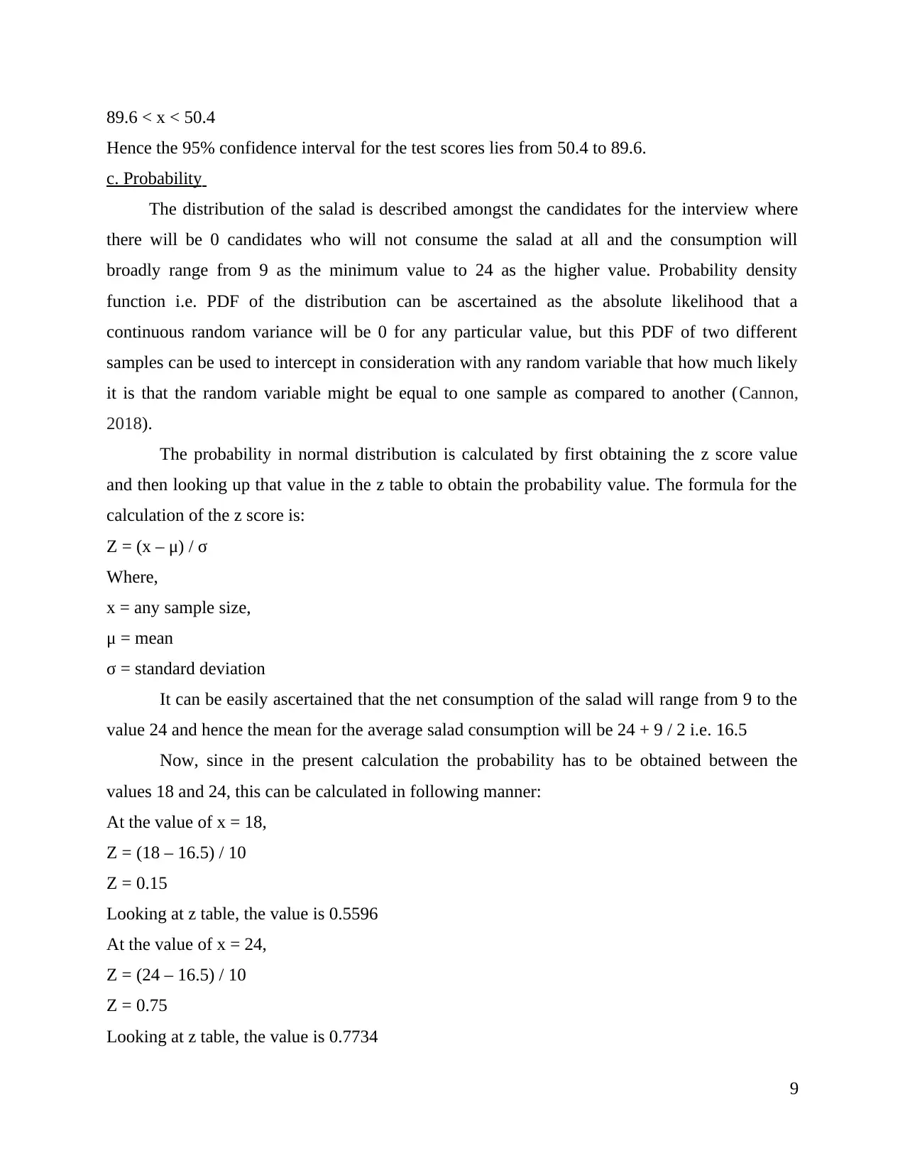
89.6 < x < 50.4
Hence the 95% confidence interval for the test scores lies from 50.4 to 89.6.
c. Probability
The distribution of the salad is described amongst the candidates for the interview where
there will be 0 candidates who will not consume the salad at all and the consumption will
broadly range from 9 as the minimum value to 24 as the higher value. Probability density
function i.e. PDF of the distribution can be ascertained as the absolute likelihood that a
continuous random variance will be 0 for any particular value, but this PDF of two different
samples can be used to intercept in consideration with any random variable that how much likely
it is that the random variable might be equal to one sample as compared to another (Cannon,
2018).
The probability in normal distribution is calculated by first obtaining the z score value
and then looking up that value in the z table to obtain the probability value. The formula for the
calculation of the z score is:
Z = (x – μ) / σ
Where,
x = any sample size,
μ = mean
σ = standard deviation
It can be easily ascertained that the net consumption of the salad will range from 9 to the
value 24 and hence the mean for the average salad consumption will be 24 + 9 / 2 i.e. 16.5
Now, since in the present calculation the probability has to be obtained between the
values 18 and 24, this can be calculated in following manner:
At the value of x = 18,
Z = (18 – 16.5) / 10
Z = 0.15
Looking at z table, the value is 0.5596
At the value of x = 24,
Z = (24 – 16.5) / 10
Z = 0.75
Looking at z table, the value is 0.7734
9

Therefore, the probability that consumption would fall between 24 and 18 is:
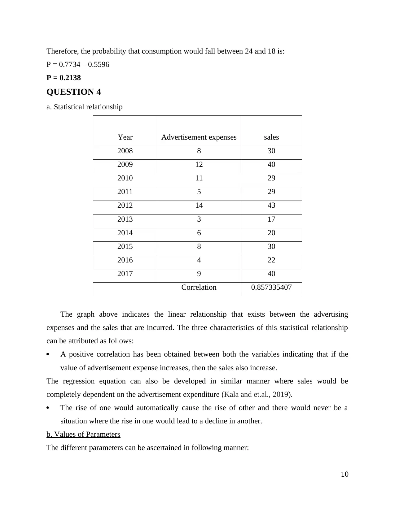
P = 0.7734 – 0.5596
P = 0.2138
QUESTION 4
a. Statistical relationship
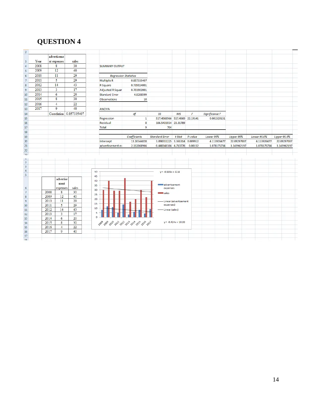
Year Advertisement expenses sales
2008 8 30
2009 12 40
2010 11 29
2011 5 29
2012 14 43
2013 3 17
2014 6 20
2015 8 30
2016 4 22
2017 9 40
Correlation 0.857335407
The graph above indicates the linear relationship that exists between the advertising
expenses and the sales that are incurred. The three characteristics of this statistical relationship
can be attributed as follows:
 A positive correlation has been obtained between both the variables indicating that if the
value of advertisement expense increases, then the sales also increase.
The regression equation can also be developed in similar manner where sales would be
completely dependent on the advertisement expenditure (Kala and et.al., 2019).
 The rise of one would automatically cause the rise of other and there would never be a
situation where the rise in one would lead to a decline in another.
b. Values of Parameters
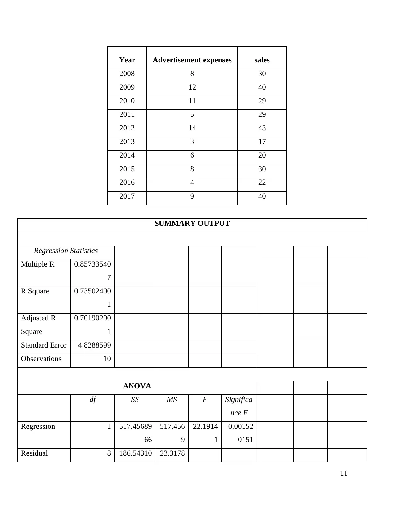
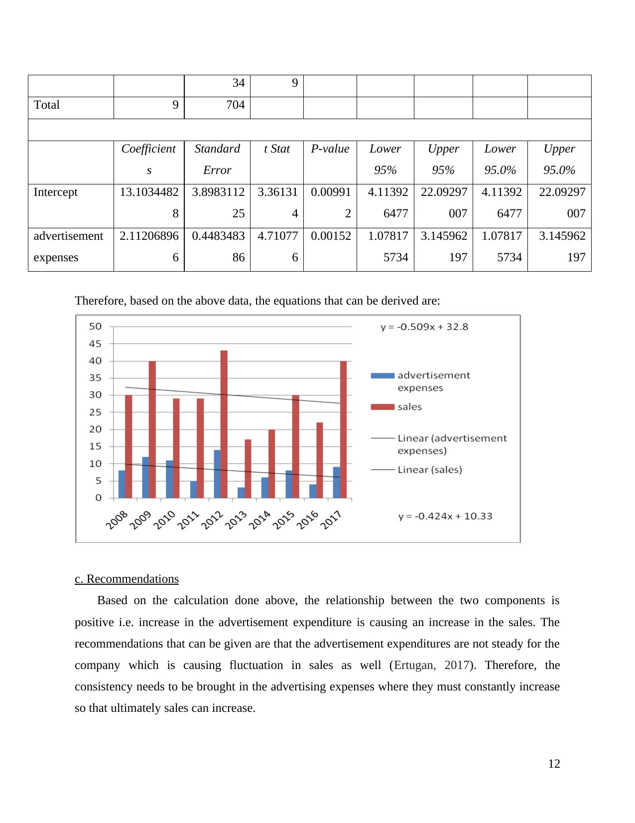
The different parameters can be ascertained in following manner:
10

Year Advertisement expenses sales
2008 8 30
2009 12 40
2010 11 29
2011 5 29
2012 14 43
2013 3 17
2014 6 20
2015 8 30
2016 4 22
2017 9 40
SUMMARY OUTPUT
Regression Statistics
Multiple R 0.85733540
7
R Square 0.73502400
1
Adjusted R
Square
0.70190200
1
Standard Error 4.8288599
Observations 10
ANOVA
df SS MS F Significa
nce F
Regression 1 517.45689
66
517.456
9
22.1914
1
0.00152
0151
Residual 8 186.54310 23.3178
11

34 9
Total 9 704
Coefficient
s
Standard
Error
t Stat P-value Lower
95%
Upper
95%
Lower
95.0%
Upper
95.0%
Intercept 13.1034482
8
3.8983112
25
3.36131
4
0.00991
2
4.11392
6477
22.09297
007
4.11392
6477
22.09297
007
advertisement
expenses
2.11206896
6
0.4483483
86
4.71077
6
0.00152 1.07817
5734
3.145962
197
1.07817
5734
3.145962
197
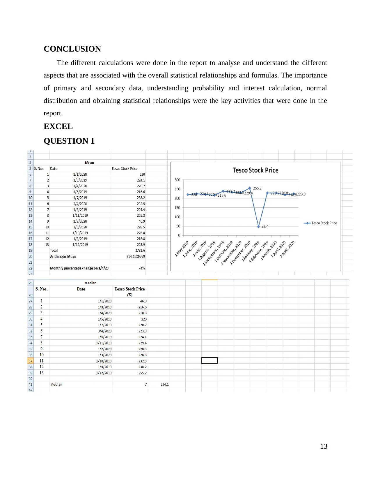
Therefore, based on the above data, the equations that can be derived are:
c. Recommendations
Based on the calculation done above, the relationship between the two components is
positive i.e. increase in the advertisement expenditure is causing an increase in the sales. The
recommendations that can be given are that the advertisement expenditures are not steady for the
company which is causing fluctuation in sales as well (Ertugan, 2017). Therefore, the
consistency needs to be brought in the advertising expenses where they must constantly increase
so that ultimately sales can increase.
12

CONCLUSION
The different calculations were done in the report to analyse and understand the different
aspects that are associated with the overall statistical relationships and formulas. The importance
of primary and secondary data, understanding probability and interest calculation, normal
distribution and obtaining statistical relationships were the key activities that were done in the
report.
EXCEL
QUESTION 1
13

QUESTION 4
14

REFERENCES
Books and Journals
Arrieta, C., Souza, R.C. and Calili, R.F., 2018. Confidence interval for the 100p-th percentile for
measurement error distributions. JPhCS, 1044(1), p.012016.
Cannon, A.J., 2018. Multivariate quantile mapping bias correction: an N-dimensional probability
density function transform for climate model simulations of multiple variables. Climate
dynamics, 50(1-2), pp.31-49.
CHAPTER, I.T., 2019. Collecting Sources. How to Write and Get Published: A Practical Guide
for Librarians, 60, p.59.
Druschke, D., and et.al., 2020. Individual-Level Linkage of Primary and Secondary Data from
Three Sources for Comprehensive Analyses of Low Birthweight Effects. Das
Gesundheitswesen, 82(S 02), pp.S108-S116.
Ertugan, A., 2017. Using statistical reasoning techniques to describe the relationship between
Facebook advertising effectiveness and benefits gained. Procedia computer science, 120,
pp.132-139.
Fishman, A. and Chai, C.K., OpenTV Inc, 2019. Collecting data from different sources. U.S.
Patent Application 16/237,022.
Johnston, M.P., 2017. Secondary data analysis: A method of which the time has
come. Qualitative and quantitative methods in libraries, 3(3), pp.619-626.
Kala, S.M., and et.al., 2019. Statistical relationship between interference estimates and network
capacity. arXiv preprint arXiv:1904.12125.
Kelkar, V., Swain, S. and Venkitesh, D., 2018. Measurement of differential modal group delay
of a few-mode fiber using a Fourier domain mode-locked laser. Optics letters, 43(9),
pp.2165-2168.
Wang, Z., 2019, December. Interference Probability Calculation Method of Frequency Agile
Radar Based on the Spectrum of Interference Signal. In 2019 Photonics &
Electromagnetics Research Symposium-Fall (PIERS-Fall) (pp. 1117-1123). IEEE.
15

16