Statistical Analysis of Non-Parametric Tests: Examples and Results
VerifiedAdded on 2022/11/01
|9
|1403
|166
Practical Assignment
AI Summary
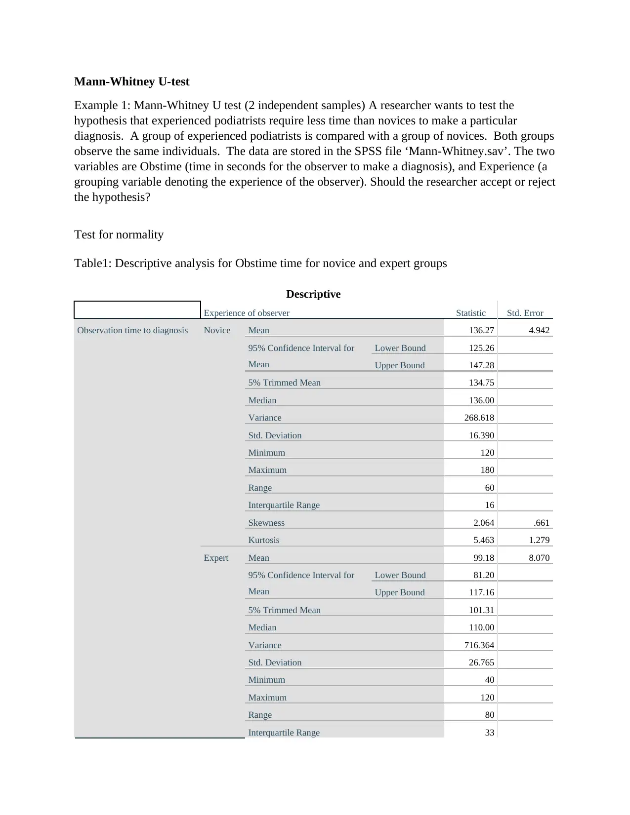
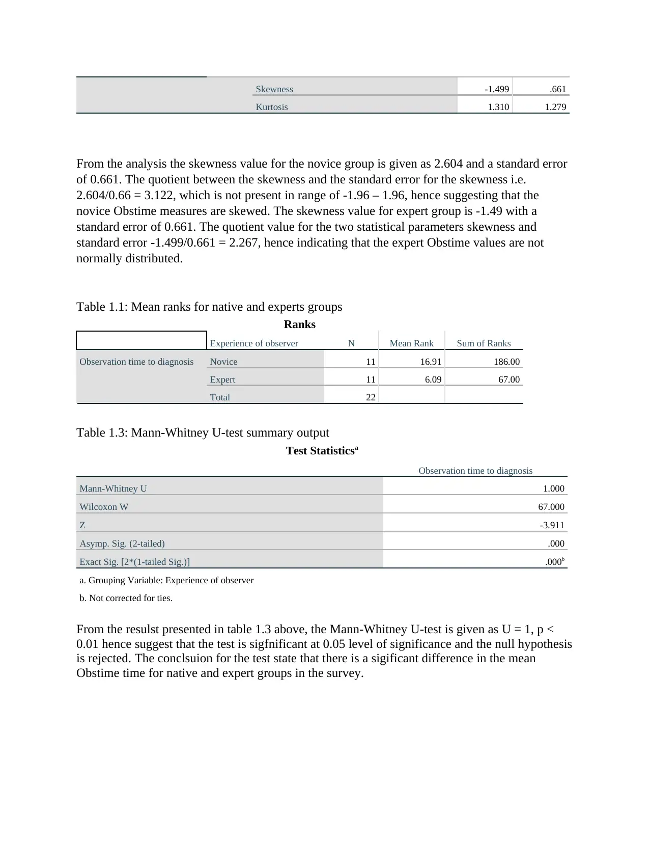
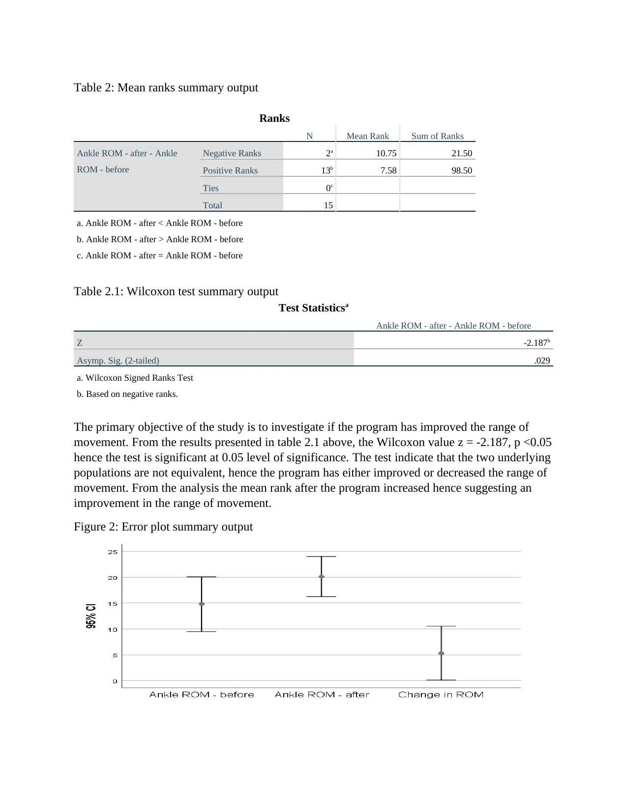
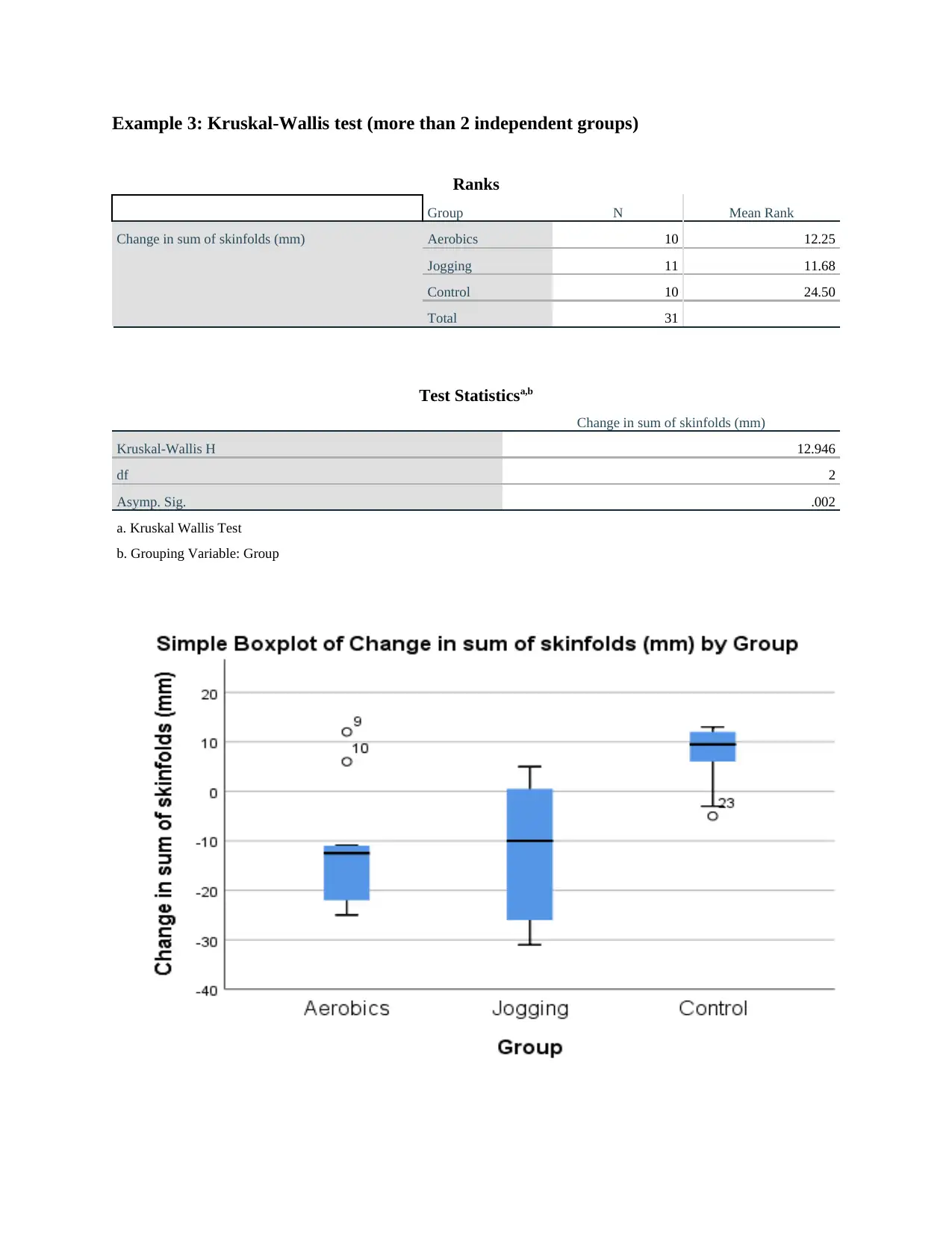
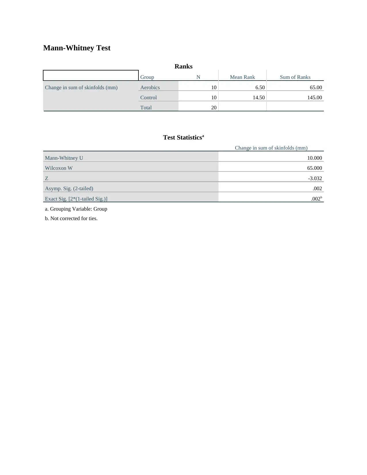
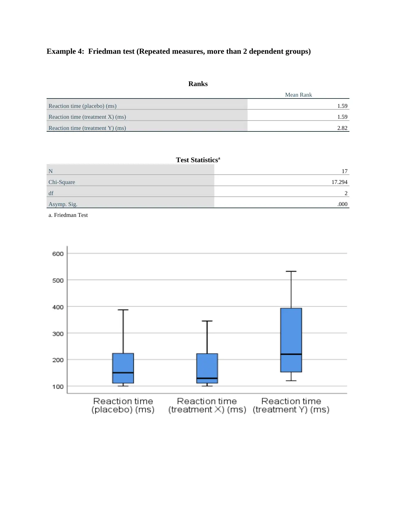
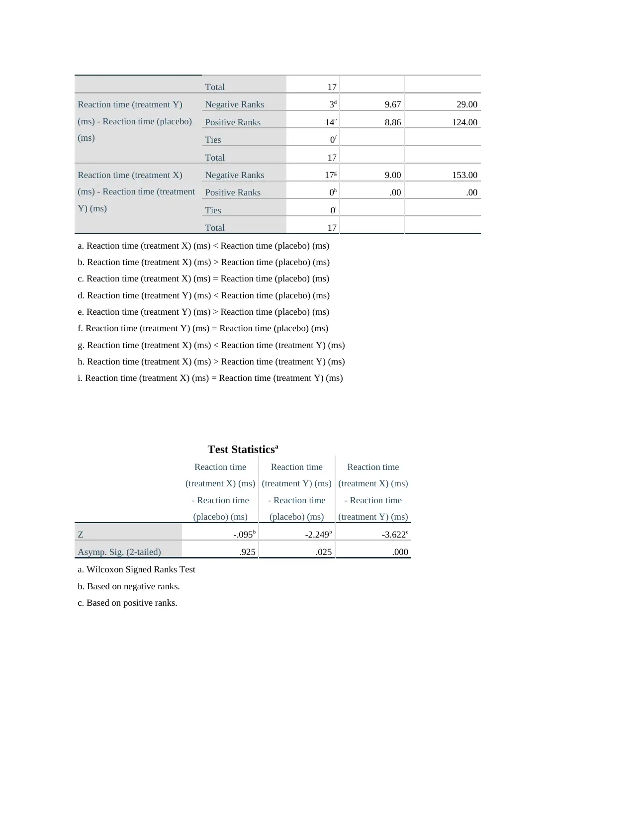
This assignment presents four examples of non-parametric statistical tests, illustrating their application and interpretation. The first example uses the Mann-Whitney U test to compare the diagnosis times of experienced and novice podiatrists, demonstrating the rejection of the null hypothesis due to a significant difference in observation times. The second example employs the Wilcoxon signed-rank test to assess the effectiveness of a new mobilization treatment on ankle range of motion, showing an improvement in range of movement after the program. The third example applies the Kruskal-Wallis test to compare changes in skinfold measurements across three groups (aerobics, jogging, and control), revealing a significant difference between the groups. Finally, the fourth example utilizes the Friedman test to analyze reaction times under different treatment conditions (placebo, treatment X, and treatment Y), indicating significant differences in reaction times among the treatments. Each example includes relevant statistical output, such as mean ranks, test statistics, and significance levels, to support the conclusions drawn about the data.

1 out of 9

Your All-in-One AI-Powered Toolkit for Academic Success.
+13062052269
info@desklib.com
Available 24*7 on WhatsApp / Email
![[object Object]](/_next/static/media/star-bottom.7253800d.svg)
Copyright © 2020–2026 A2Z Services. All Rights Reserved. Developed and managed by ZUCOL.