Research on Introduction 2022

Introduction
In today’s world each and every company or factory struggles to reduce the cost of production
and meet the customer’s needs. The car manufacturing industries based in USA conducted a
research to analyze whether they could produce cars types or models that would consume less
fuel. This research was carried out using different features such as number of cylinders in the car,
horse power of the engine, galloons per hundred miles, weight in 100 1b and last but not least the
seconds taken to arrive at a speed from zero to sixty miles. Some of the analysis carried out
involves association (correlation) between the variables.
Results and Discussions
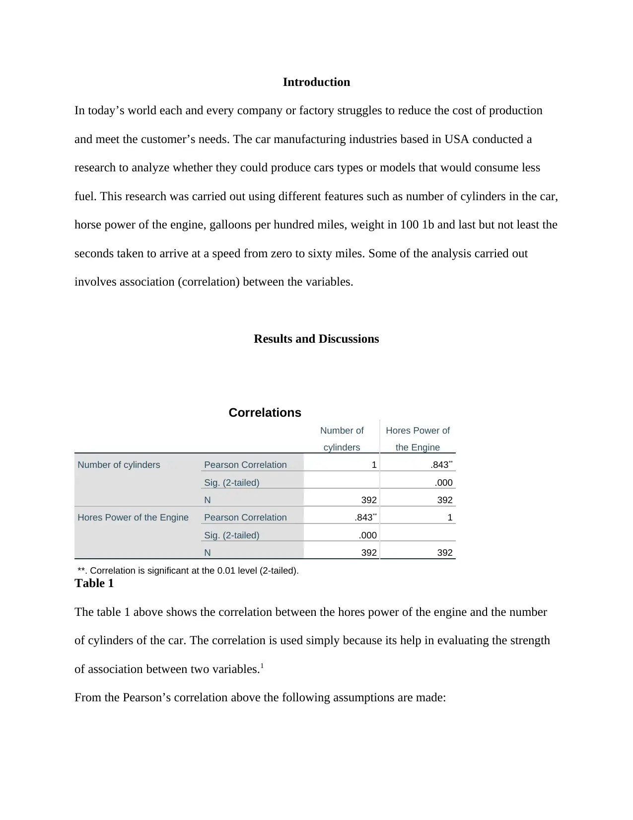
Correlations
Number of
cylinders
Hores Power of
the Engine
Number of cylinders Pearson Correlation 1 .843**
Sig. (2-tailed) .000
N 392 392
Hores Power of the Engine Pearson Correlation .843** 1
Sig. (2-tailed) .000
N 392 392
**. Correlation is significant at the 0.01 level (2-tailed).
Table 1
The table 1 above shows the correlation between the hores power of the engine and the number
of cylinders of the car. The correlation is used simply because its help in evaluating the strength
of association between two variables.1
From the Pearson’s correlation above the following assumptions are made:

 The normality of the data set that is the data set that ought to be correlated should
approximate the normal distribution. The data point tends to be close to the mean.
 We also assume that the error term or variance size of the variable number of cylinder
and the horse power of the engine should have equal values that are homoscedascity
should not be violated.
 We further assume that there is a linear relationship between the variables. This can be
investigated by plotting a scatter plot and fitting with a line of best fit. Therefore, if a
straight line is obtained then the assumption holds true.
 The two variables are also assumed to be continuous that is the variables are either ratio
or scale.
 Another assumption considered is that the two variables should contain data point that are
equal that is every data point of the number of cylinders should correspond to the data
point of the variable the horse power of the engine.
From the table 1 above, we observe that the Pearson correlation between the number of cylinders
and hores power of the engine of the car is 0.843. The Pearson correlation of number of cylinders
by itself is 1. In addition, the Pearson correlation between the hores power of the engine and
itself is also 1. The total values used in this analysis are 392 with no missing value. The p-value
is also given as 0.000 which is indicated as sig. two-tailed.
The Pearson correlation between the number of cylinders and hores power of the engine is
strongly positive showing that the two variables tends to increase together. The p-value is also
less than the statistical significance value of 0.01 hence the null hypothesis is rejected and
conclusion made on the alternative hypothesis. Therefore, there exists a correlation between the
two variables.

Model Summary
Model R R Square
Adjusted R
Square
Std. Error of the
Estimate
1 .883a .779 .778 .78600
a. Predictors: (Constant), Hores Power of the Engine, Number of
cylinders
ANOVAa
Model Sum of Squares df Mean Square F Sig.
1 Regression 848.363 2 424.182 686.598 .000b
Residual 240.325 389 .618
Total 1088.688 391
a. Dependent Variable: GallonsPer100Miles
b. Predictors: (Constant), Hores Power of the Engine, Number of cylinders
Coefficientsa
Model
Unstandardized Coefficients
Standardized
Coefficients
t Sig.B Std. Error Beta
1 (Constant) .280 .134 2.094 .037
Number of cylinders .406 .043 .415 9.374 .000
Hores Power of the Engine 2.185 .192 .504 11.383 .000
a. Dependent Variable: GallonsPer100Miles
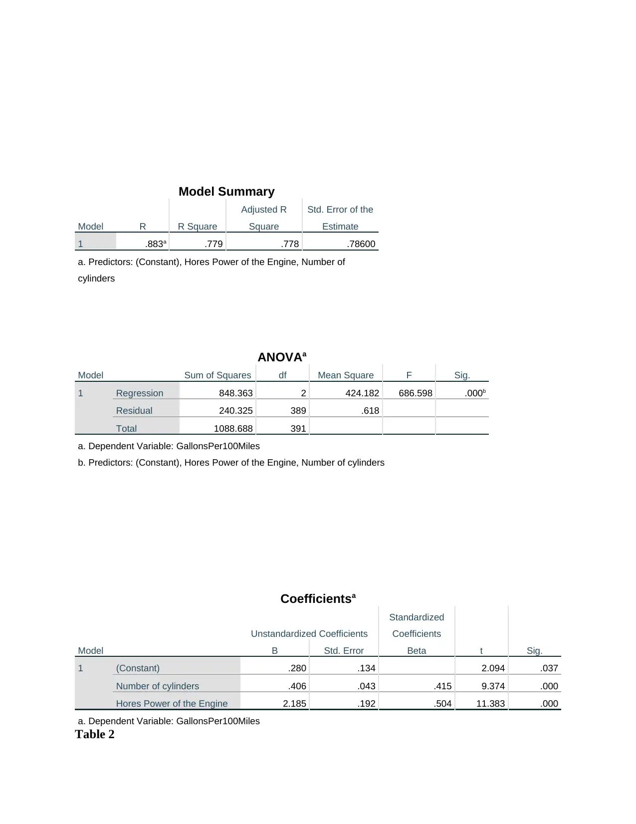
Table 2

From the table 2 above, a linear regression analysis has been conducted on the variable such as
number of cylinder and horse power of the engine and the gallons per 100 miles. All these
variables have been grouped into the dependent variable (gallons per 100 miles, the number of
cylinders and horse power of the engine are independent variables. The reason to why a linear is
used is because the goal of the research is to determine whether the number of cylinders and
horse power of the engine would lead to high fuel consumption.2 Furthermore, the study also
finds out whether the number of cylinders has a great influence on fuel consumption compared to
the horse power of the engine. The above regression model has the following vital assumptions:
 Linear association or relationship
 Little or no multicollinearity
 Existence of a normality referred to us multivariate
 Existence of none auto- correlation
 Existence of homoscedasticity
The data sets provided in SPSS that have been used to generate the above regression model have
not violated the above assumptions. For instance, both the variables that are number of cylinders
and horse power of the engine are linearly correlated. This has been has been analyzed above
using the correlation. From the model above there is little multicollinearity, this can be
investigated using the coefficient of the independent variable. This will be discussed in detail
when interpreting the results. Using the SPSS software we can use Durbin-Watson to investigate
the linear auto-correlation in the data set. Furthermore, the homoscedasticity and multivariate
normality can be analyzed well in SPSS using the Q-Q-plot.

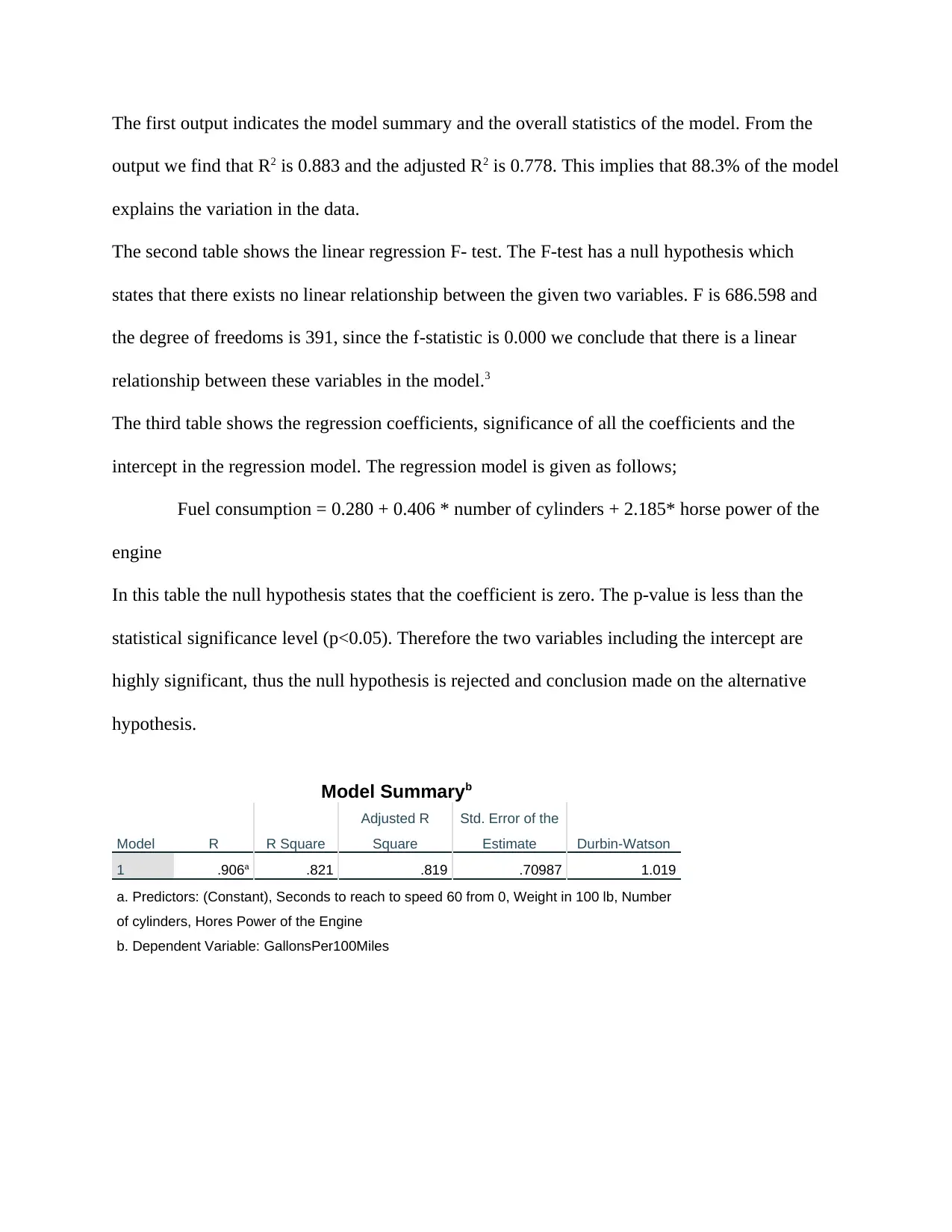
The first output indicates the model summary and the overall statistics of the model. From the
output we find that R2 is 0.883 and the adjusted R2 is 0.778. This implies that 88.3% of the model
explains the variation in the data.
The second table shows the linear regression F- test. The F-test has a null hypothesis which
states that there exists no linear relationship between the given two variables. F is 686.598 and
the degree of freedoms is 391, since the f-statistic is 0.000 we conclude that there is a linear
relationship between these variables in the model.3
The third table shows the regression coefficients, significance of all the coefficients and the
intercept in the regression model. The regression model is given as follows;
Fuel consumption = 0.280 + 0.406 * number of cylinders + 2.185* horse power of the
engine
In this table the null hypothesis states that the coefficient is zero. The p-value is less than the
statistical significance level (p<0.05). Therefore the two variables including the intercept are
highly significant, thus the null hypothesis is rejected and conclusion made on the alternative
hypothesis.
Model Summaryb
Model R R Square
Adjusted R
Square
Std. Error of the
Estimate Durbin-Watson
1 .906a .821 .819 .70987 1.019
a. Predictors: (Constant), Seconds to reach to speed 60 from 0, Weight in 100 lb, Number
of cylinders, Hores Power of the Engine
b. Dependent Variable: GallonsPer100Miles

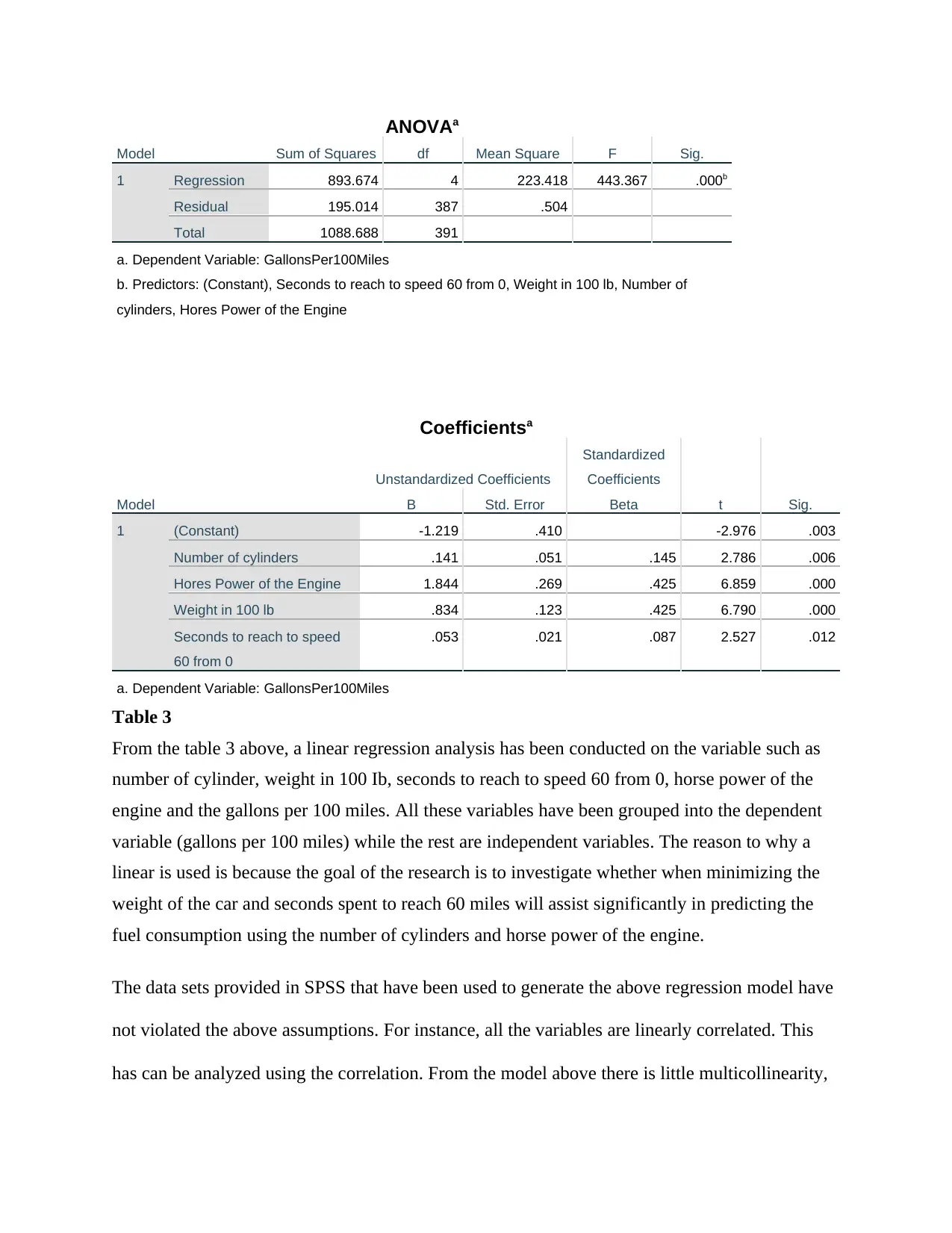
ANOVAa
Model Sum of Squares df Mean Square F Sig.
1 Regression 893.674 4 223.418 443.367 .000b
Residual 195.014 387 .504
Total 1088.688 391
a. Dependent Variable: GallonsPer100Miles
b. Predictors: (Constant), Seconds to reach to speed 60 from 0, Weight in 100 lb, Number of
cylinders, Hores Power of the Engine
Coefficientsa
Model
Unstandardized Coefficients
Standardized
Coefficients
t Sig.B Std. Error Beta
1 (Constant) -1.219 .410 -2.976 .003
Number of cylinders .141 .051 .145 2.786 .006
Hores Power of the Engine 1.844 .269 .425 6.859 .000
Weight in 100 lb .834 .123 .425 6.790 .000
Seconds to reach to speed
60 from 0
.053 .021 .087 2.527 .012
a. Dependent Variable: GallonsPer100Miles
Table 3
From the table 3 above, a linear regression analysis has been conducted on the variable such as
number of cylinder, weight in 100 Ib, seconds to reach to speed 60 from 0, horse power of the
engine and the gallons per 100 miles. All these variables have been grouped into the dependent
variable (gallons per 100 miles) while the rest are independent variables. The reason to why a
linear is used is because the goal of the research is to investigate whether when minimizing the
weight of the car and seconds spent to reach 60 miles will assist significantly in predicting the
fuel consumption using the number of cylinders and horse power of the engine.
The data sets provided in SPSS that have been used to generate the above regression model have
not violated the above assumptions. For instance, all the variables are linearly correlated. This
has can be analyzed using the correlation. From the model above there is little multicollinearity,

this can be investigated using the coefficient of the independent variable. This will be discussed
in detail when interpreting the results. Using the SPSS software we can use Durbin-Watson to
investigate the linear auto-correlation in the data set. Furthermore, the homoscedasticity and
multivariate normality can be analyzed well in SPSS using the Q-Q-plot.
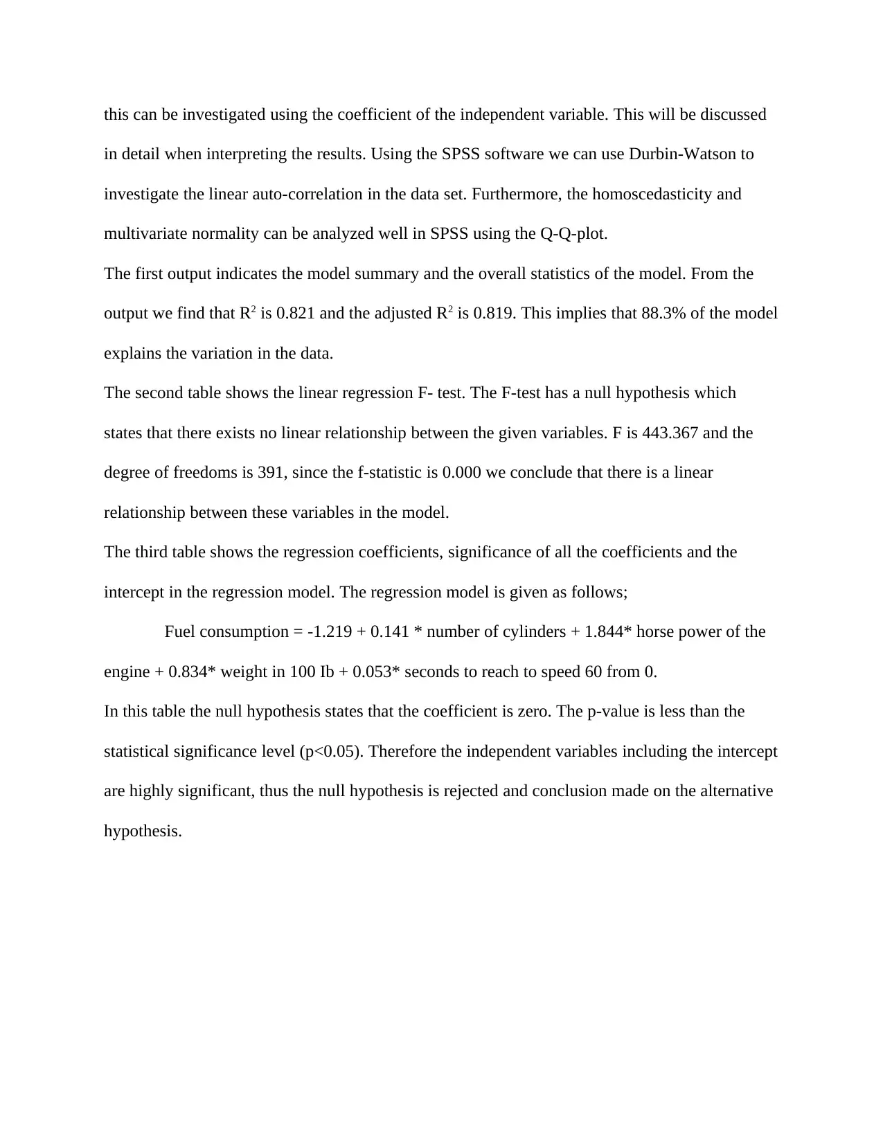
The first output indicates the model summary and the overall statistics of the model. From the
output we find that R2 is 0.821 and the adjusted R2 is 0.819. This implies that 88.3% of the model
explains the variation in the data.
The second table shows the linear regression F- test. The F-test has a null hypothesis which
states that there exists no linear relationship between the given variables. F is 443.367 and the
degree of freedoms is 391, since the f-statistic is 0.000 we conclude that there is a linear
relationship between these variables in the model.
The third table shows the regression coefficients, significance of all the coefficients and the
intercept in the regression model. The regression model is given as follows;
Fuel consumption = -1.219 + 0.141 * number of cylinders + 1.844* horse power of the
engine + 0.834* weight in 100 Ib + 0.053* seconds to reach to speed 60 from 0.
In this table the null hypothesis states that the coefficient is zero. The p-value is less than the
statistical significance level (p<0.05). Therefore the independent variables including the intercept
are highly significant, thus the null hypothesis is rejected and conclusion made on the alternative
hypothesis.

Bibliography

1 . Kenett, Dror Y., Xuqing Huang, Irena Vodenska, Shlomo Havlin, and H. Eugene Stanley.
"Partial correlation analysis: Applications for financial markets." Quantitative Finance 15,
no. 4 (2015): 569-578.
2 . Austin, Peter C., and Ewout W. Steyerberg. "The number of subjects per variable required
in linear regression analyses." Journal of clinical epidemiology 68, no. 6 (2015): 627-636.
3 . Jann, Ben. Influence functions for linear regression (with an application to regression
adjustment). No. 32. University of Bern, Department of Social Sciences, 2019.