Microeconomics and Profit Maximization
VerifiedAdded on 2020/05/28
|16
|1897
|399
AI Summary
This assignment delves into the core concepts of microeconomics, focusing on a firm's objective of maximizing profit. It explores two approaches to achieving this goal: the total revenue-total cost method and the marginal revenue-marginal cost method. The assignment explains how these methods work, using graphs and examples to illustrate the concepts. Students will learn about elasticity, price determination, and the factors influencing a firm's profit-maximizing output.
Contribute Materials
Your contribution can guide someone’s learning journey. Share your
documents today.
Running Head: ECONOMIC ASSIGNMENT
Economic Assignment
Name of the Student
Name of the University
Author note
Economic Assignment
Name of the Student
Name of the University
Author note
Secure Best Marks with AI Grader
Need help grading? Try our AI Grader for instant feedback on your assignments.
1ECONOMIC ASSIGNMENT
Table of Contents
Answer 1..........................................................................................................................................2
Answer a......................................................................................................................................2
Answer b......................................................................................................................................3
Answer 2..........................................................................................................................................4
Answer a......................................................................................................................................4
Answer b......................................................................................................................................5
Answer c......................................................................................................................................6
Answer 3..........................................................................................................................................8
Answer 4........................................................................................................................................10
Answer a....................................................................................................................................10
Answer b....................................................................................................................................11
Answer 5........................................................................................................................................12
References......................................................................................................................................15
2ECONOMIC ASSIGNMENT
Answer 1
Answer a
An increase in petrol prices arising from global supply shortage of petrol has a direct
impact on petrol demand. When price increases, then quantity demand for petrol reduces (Frank
2014). As a result, they chose to buy cars that are fuel-efficient that requires less amount of
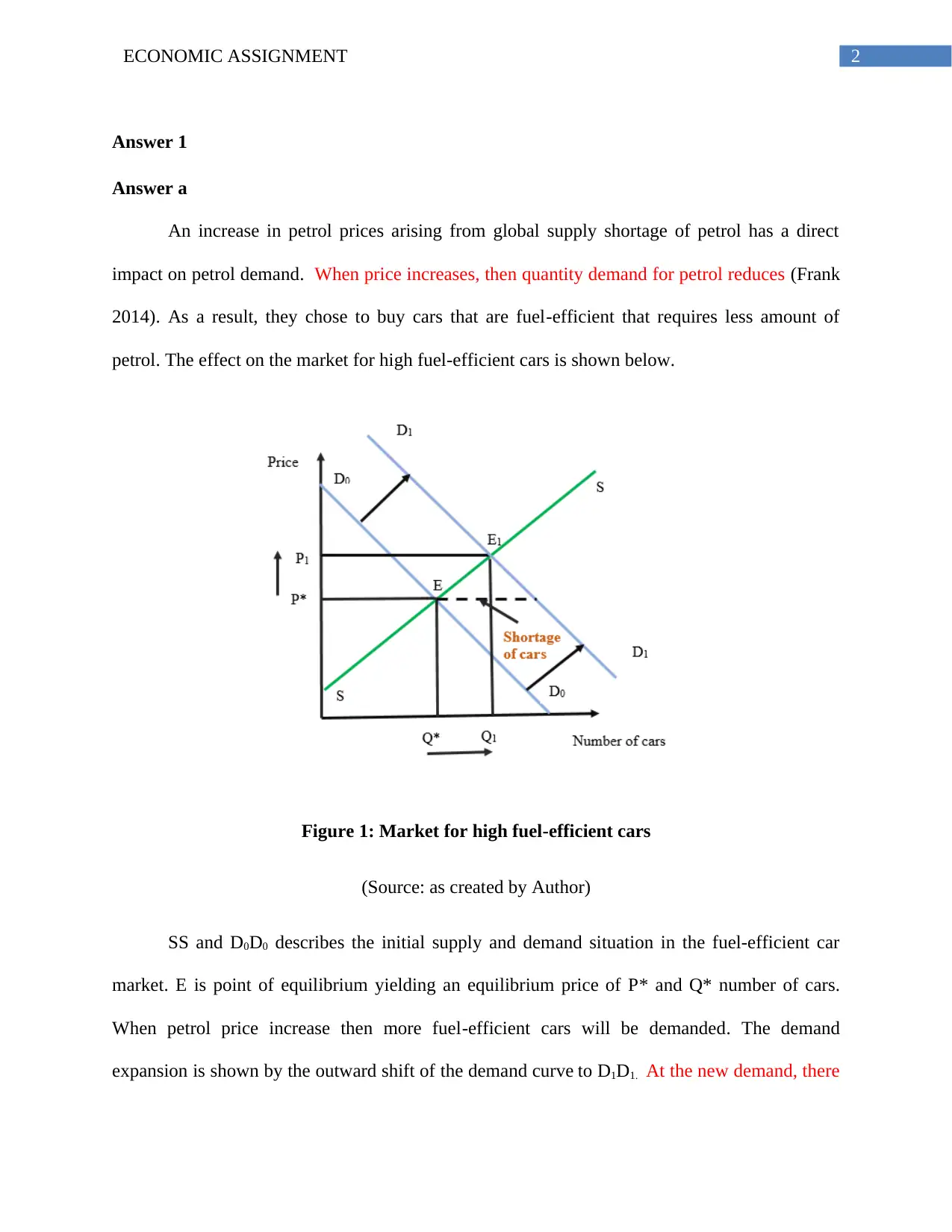
petrol. The effect on the market for high fuel-efficient cars is shown below.
Figure 1: Market for high fuel-efficient cars
(Source: as created by Author)
SS and D0D0 describes the initial supply and demand situation in the fuel-efficient car
market. E is point of equilibrium yielding an equilibrium price of P* and Q* number of cars.
When petrol price increase then more fuel-efficient cars will be demanded. The demand
expansion is shown by the outward shift of the demand curve to D1D1. At the new demand, there
3ECONOMIC ASSIGNMENT
will be a shortage of fuel-efficient cars. The new equilibrium is at the intersection point of new
demand curve D1D1 and old supply curve SS. E1 is the new equilibrium point where price has
increased to P1 and number of cars increased to Q1.
Answer b
The effect of petrol price increase in the market for petro-substitutes products such as
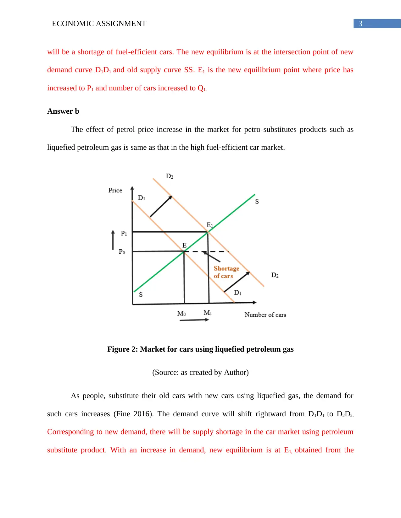
liquefied petroleum gas is same as that in the high fuel-efficient car market.
Figure 2: Market for cars using liquefied petroleum gas
(Source: as created by Author)
As people, substitute their old cars with new cars using liquefied gas, the demand for
such cars increases (Fine 2016). The demand curve will shift rightward from D1D1 to D2D2.
Corresponding to new demand, there will be supply shortage in the car market using petroleum
substitute product. With an increase in demand, new equilibrium is at E1, obtained from the
Secure Best Marks with AI Grader
Need help grading? Try our AI Grader for instant feedback on your assignments.
4ECONOMIC ASSIGNMENT
intersection of D2D2 and existing supply curve SS. Consequently, in the new equilibrium there is
a rise in price from P0 to P1 with an increase in number of cars sold from M0 to M1.
Answer 2
Answer a
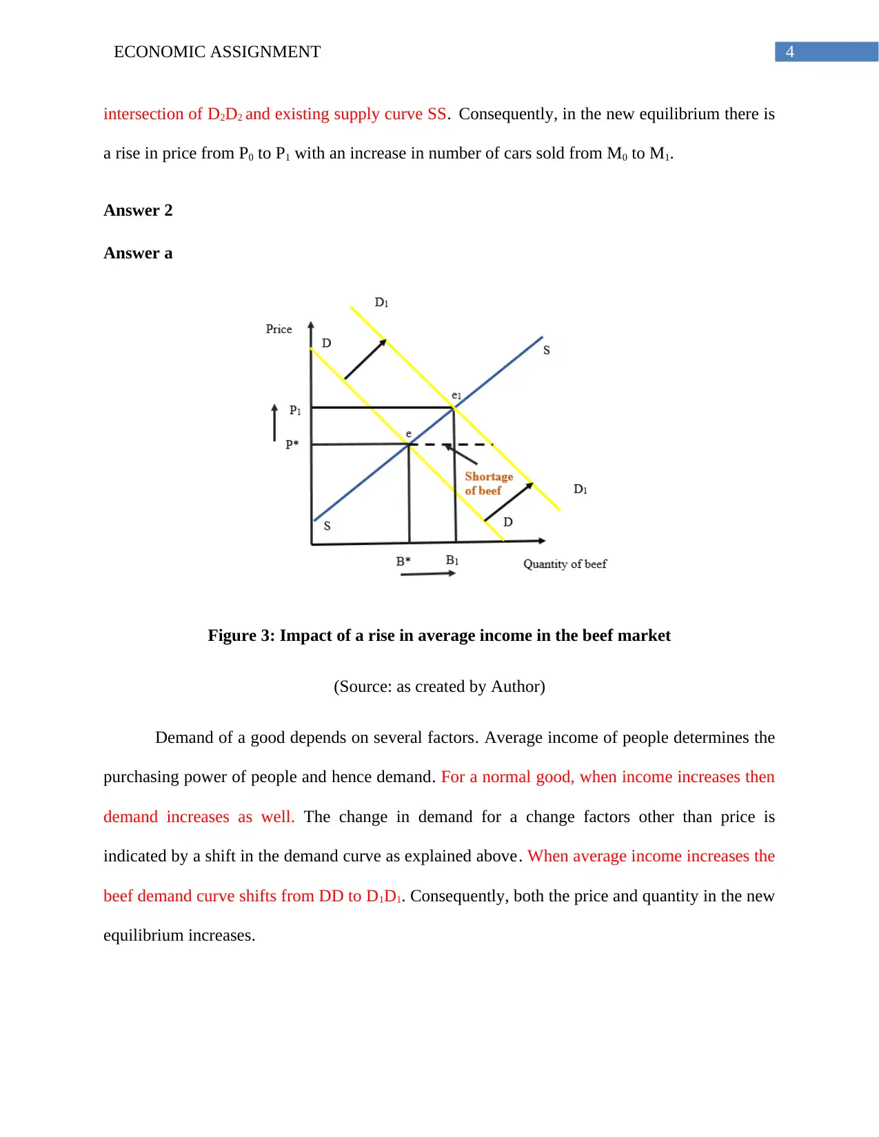
Figure 3: Impact of a rise in average income in the beef market
(Source: as created by Author)
Demand of a good depends on several factors. Average income of people determines the
purchasing power of people and hence demand. For a normal good, when income increases then
demand increases as well. The change in demand for a change factors other than price is
indicated by a shift in the demand curve as explained above. When average income increases the
beef demand curve shifts from DD to D1D1. Consequently, both the price and quantity in the new
equilibrium increases.
5ECONOMIC ASSIGNMENT
Answer b
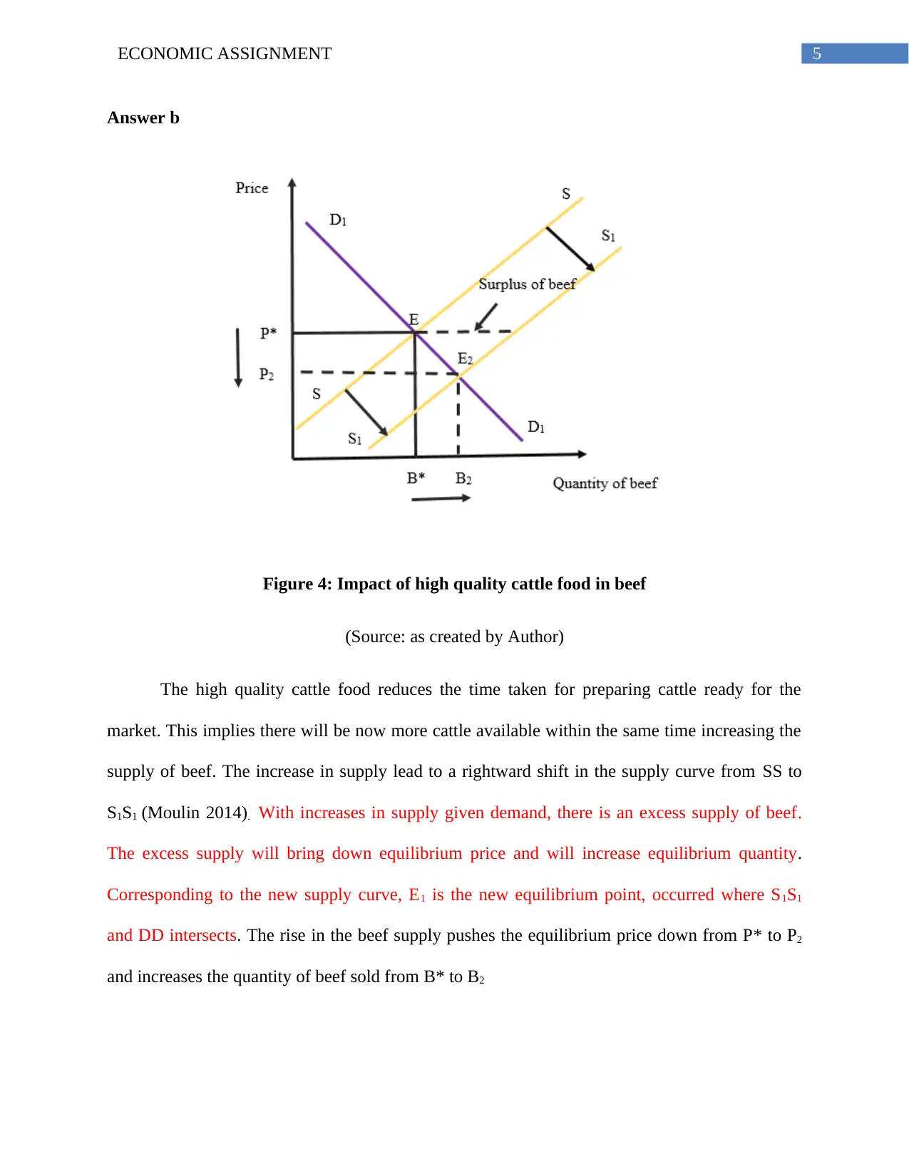
Figure 4: Impact of high quality cattle food in beef
(Source: as created by Author)
The high quality cattle food reduces the time taken for preparing cattle ready for the
market. This implies there will be now more cattle available within the same time increasing the
supply of beef. The increase in supply lead to a rightward shift in the supply curve from SS to
S1S1 (Moulin 2014). With increases in supply given demand, there is an excess supply of beef.
The excess supply will bring down equilibrium price and will increase equilibrium quantity.
Corresponding to the new supply curve, E1 is the new equilibrium point, occurred where S1S1
and DD intersects. The rise in the beef supply pushes the equilibrium price down from P* to P2
and increases the quantity of beef sold from B* to B2
6ECONOMIC ASSIGNMENT
Answer c
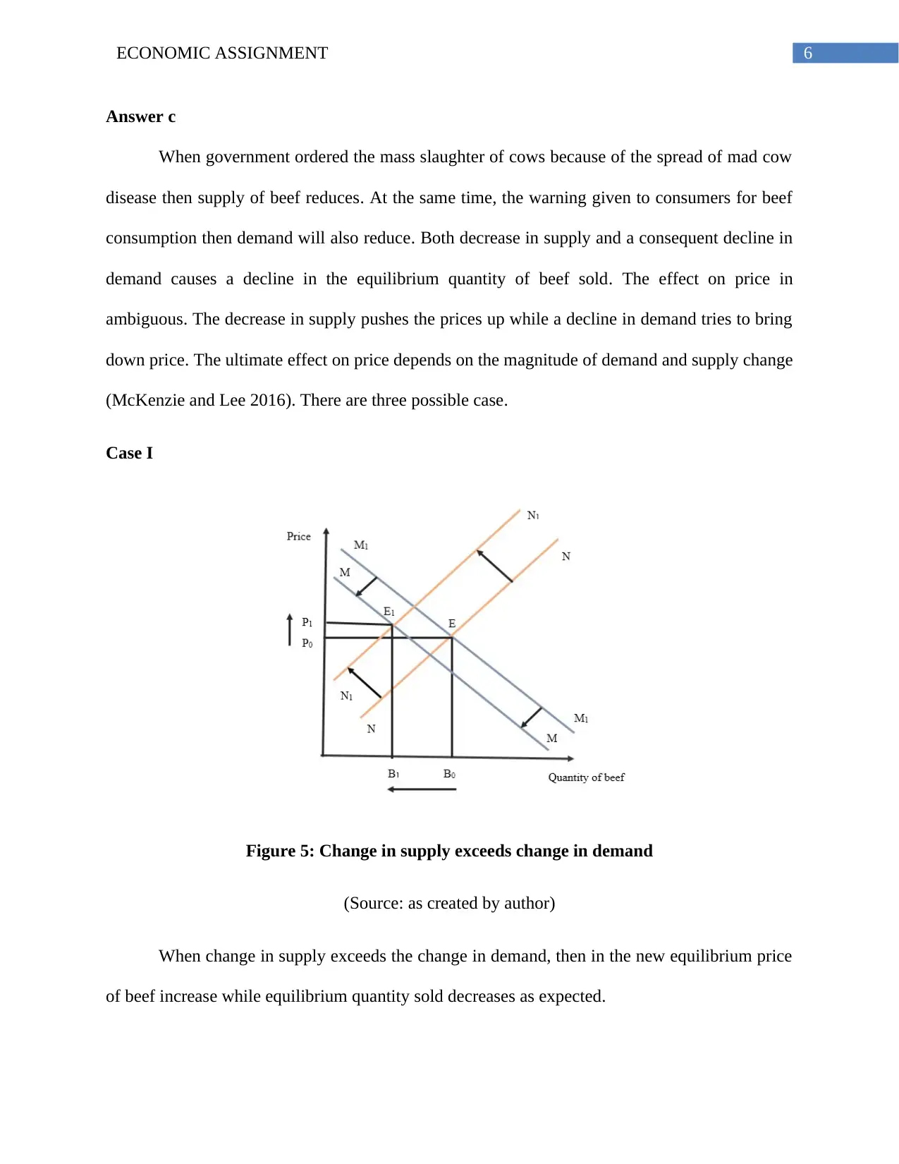
When government ordered the mass slaughter of cows because of the spread of mad cow
disease then supply of beef reduces. At the same time, the warning given to consumers for beef
consumption then demand will also reduce. Both decrease in supply and a consequent decline in
demand causes a decline in the equilibrium quantity of beef sold. The effect on price in
ambiguous. The decrease in supply pushes the prices up while a decline in demand tries to bring
down price. The ultimate effect on price depends on the magnitude of demand and supply change
(McKenzie and Lee 2016). There are three possible case.
Case I
Figure 5: Change in supply exceeds change in demand
(Source: as created by author)
When change in supply exceeds the change in demand, then in the new equilibrium price
of beef increase while equilibrium quantity sold decreases as expected.
Paraphrase This Document
Need a fresh take? Get an instant paraphrase of this document with our AI Paraphraser
7ECONOMIC ASSIGNMENT
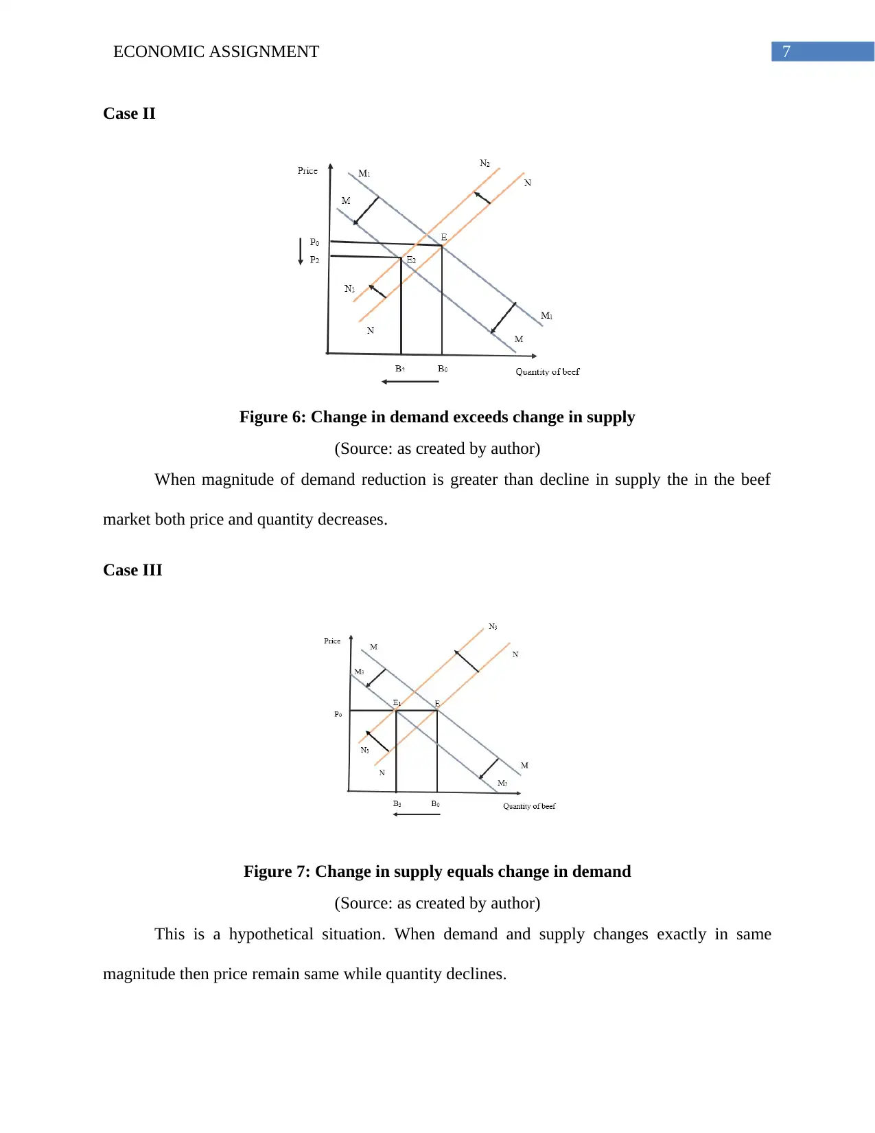
Case II
Figure 6: Change in demand exceeds change in supply
(Source: as created by author)
When magnitude of demand reduction is greater than decline in supply the in the beef
market both price and quantity decreases.
Case III
Figure 7: Change in supply equals change in demand
(Source: as created by author)
This is a hypothetical situation. When demand and supply changes exactly in same
magnitude then price remain same while quantity declines.
8ECONOMIC ASSIGNMENT
Answer 3
The increases in new commercial apartment combines with a decrease in availability of
such apartment. This means in the housing market, there occur a change in both supply and
demand. An increase supply causes a decrease in price. The reduced demand also has the same
impact on price (Elsner, Heinrich and Schwardt 2014). However, the effect of equilibrium
number of houses is ambiguous. The supply forces tend to increase number of such apartments
while demand forces causes a decline equilibrium number of apartments. The final impact on the
number of apartments is subject to magnitude of changes in demand and supply.
Case I
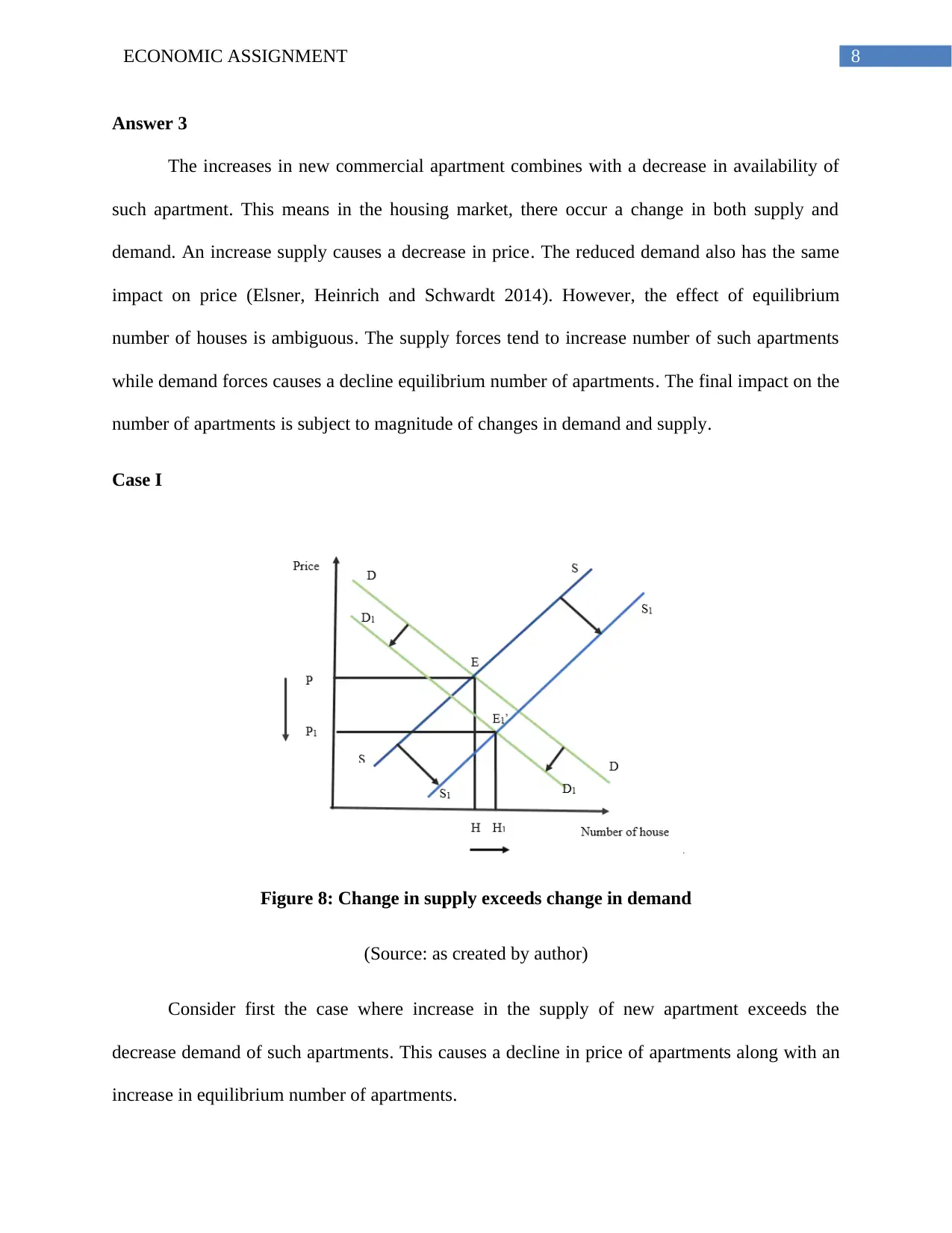
Figure 8: Change in supply exceeds change in demand
(Source: as created by author)
Consider first the case where increase in the supply of new apartment exceeds the
decrease demand of such apartments. This causes a decline in price of apartments along with an
increase in equilibrium number of apartments.
9ECONOMIC ASSIGNMENT
Case II
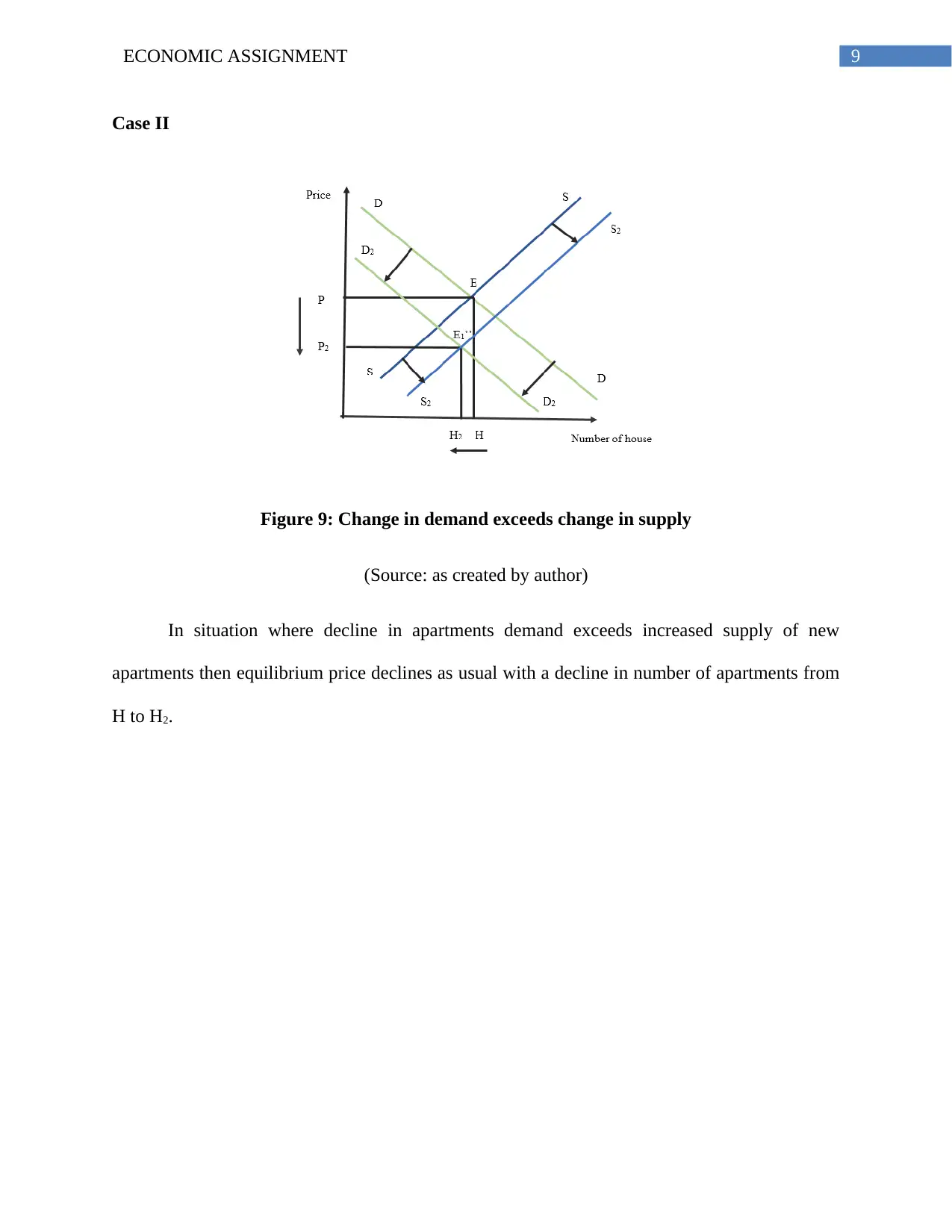
Figure 9: Change in demand exceeds change in supply
(Source: as created by author)
In situation where decline in apartments demand exceeds increased supply of new
apartments then equilibrium price declines as usual with a decline in number of apartments from
H to H2.
Case II
Figure 9: Change in demand exceeds change in supply
(Source: as created by author)
In situation where decline in apartments demand exceeds increased supply of new
apartments then equilibrium price declines as usual with a decline in number of apartments from
H to H2.
Secure Best Marks with AI Grader
Need help grading? Try our AI Grader for instant feedback on your assignments.
10ECONOMIC ASSIGNMENT
Case III
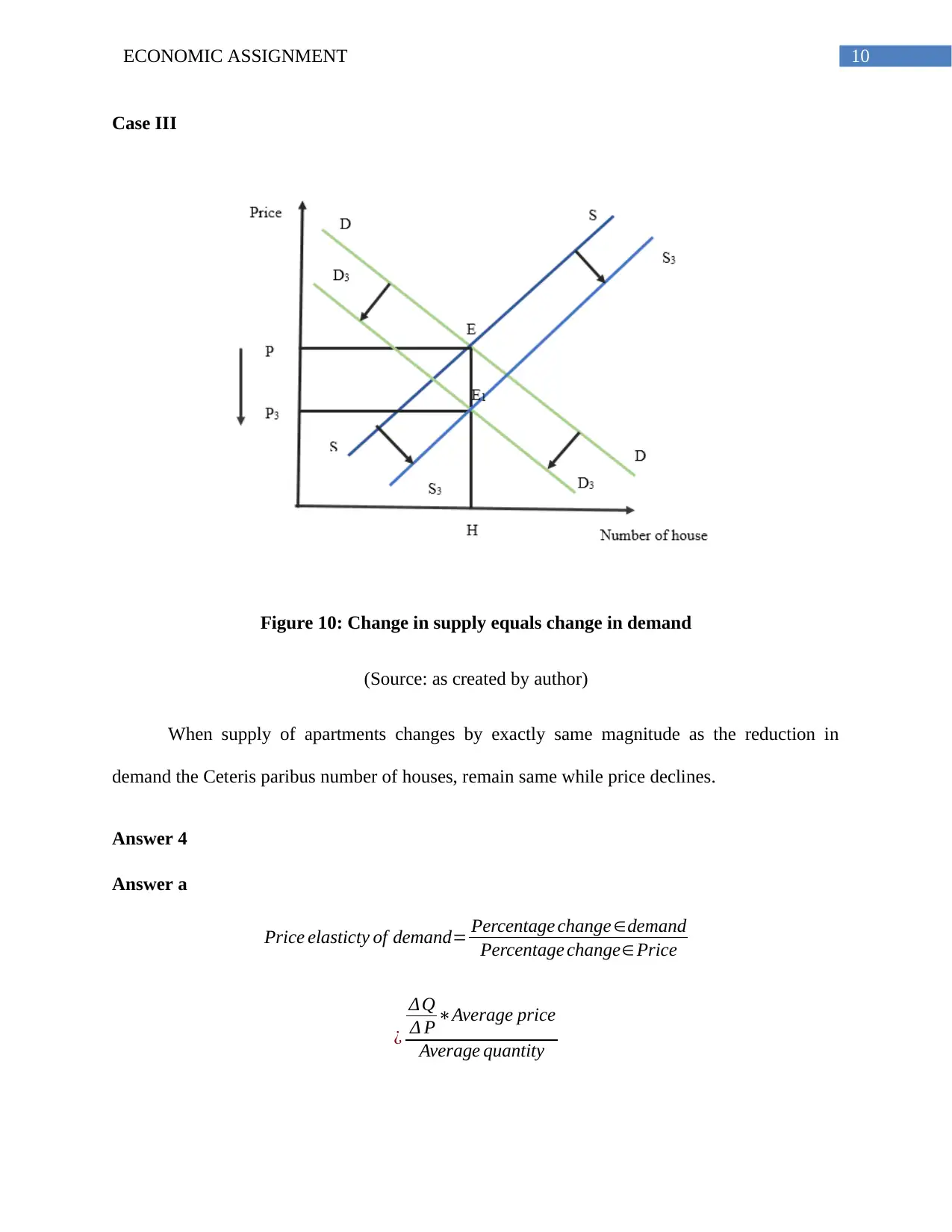
Figure 10: Change in supply equals change in demand
(Source: as created by author)
When supply of apartments changes by exactly same magnitude as the reduction in
demand the Ceteris paribus number of houses, remain same while price declines.
Answer 4
Answer a
Price elasticty of demand= Percentage change ∈demand
Percentage change∈ Price
¿
ΔQ
Δ P ∗Average price
Average quantity
11ECONOMIC ASSIGNMENT
¿
(Q2−Q1)
( P2−P1) ∗( P1 + P2)/2
(Q1 +Q2)/2
¿
(15−25)
(4 . 25−3 .50)∗(3 .50+ 4 . 25)/2
(25+ 15)/2
¿
−10
0 . 75∗3 . 875
20
¿−13 .33∗0 . 194
¿−2 .586 −2 .59
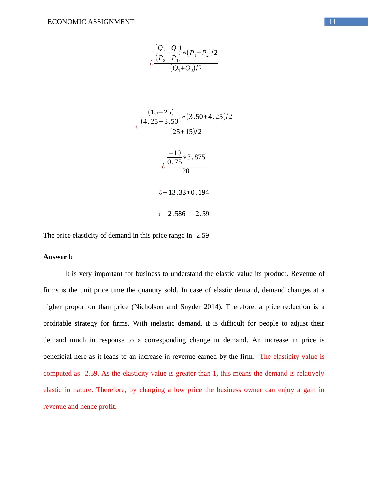
The price elasticity of demand in this price range in -2.59.
Answer b
It is very important for business to understand the elastic value its product. Revenue of
firms is the unit price time the quantity sold. In case of elastic demand, demand changes at a
higher proportion than price (Nicholson and Snyder 2014). Therefore, a price reduction is a
profitable strategy for firms. With inelastic demand, it is difficult for people to adjust their
demand much in response to a corresponding change in demand. An increase in price is
beneficial here as it leads to an increase in revenue earned by the firm. The elasticity value is
computed as -2.59. As the elasticity value is greater than 1, this means the demand is relatively
elastic in nature. Therefore, by charging a low price the business owner can enjoy a gain in
revenue and hence profit.
¿
(Q2−Q1)
( P2−P1) ∗( P1 + P2)/2
(Q1 +Q2)/2
¿
(15−25)
(4 . 25−3 .50)∗(3 .50+ 4 . 25)/2
(25+ 15)/2
¿
−10
0 . 75∗3 . 875
20
¿−13 .33∗0 . 194
¿−2 .586 −2 .59
The price elasticity of demand in this price range in -2.59.
Answer b
It is very important for business to understand the elastic value its product. Revenue of
firms is the unit price time the quantity sold. In case of elastic demand, demand changes at a
higher proportion than price (Nicholson and Snyder 2014). Therefore, a price reduction is a
profitable strategy for firms. With inelastic demand, it is difficult for people to adjust their
demand much in response to a corresponding change in demand. An increase in price is
beneficial here as it leads to an increase in revenue earned by the firm. The elasticity value is
computed as -2.59. As the elasticity value is greater than 1, this means the demand is relatively
elastic in nature. Therefore, by charging a low price the business owner can enjoy a gain in
revenue and hence profit.
12ECONOMIC ASSIGNMENT
Answer 5
Objective of a firm is to maximize profit. Profit is obtained as a difference between total
revenue and total cost.
Profit = Total Revenue (TR) – Total Cost (TC)
There are two approaches towards profit maximizing decision. One is Total revenue-total cost
method and other is marginal revenue-marginal cost method.
Total Revenue –total cost method
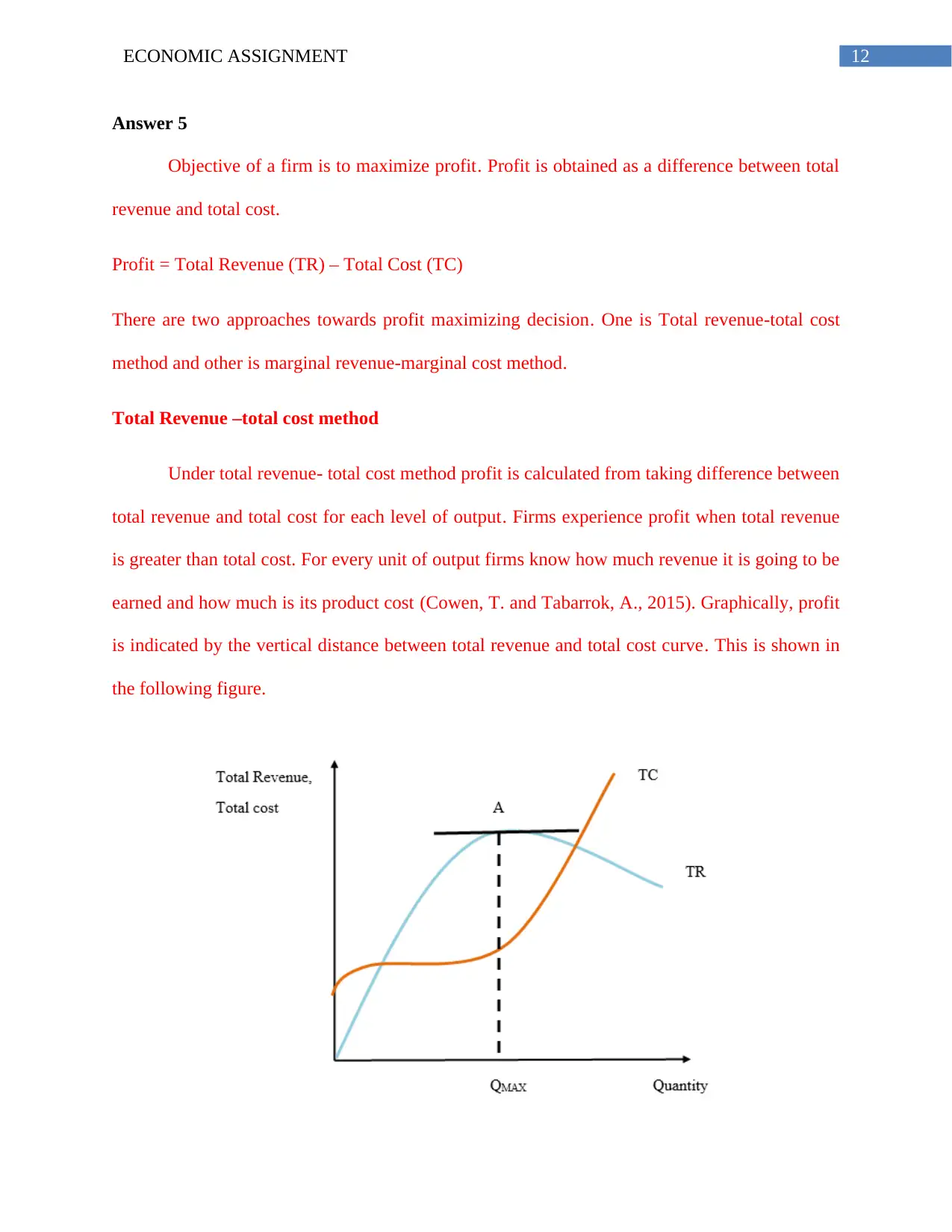
Under total revenue- total cost method profit is calculated from taking difference between
total revenue and total cost for each level of output. Firms experience profit when total revenue
is greater than total cost. For every unit of output firms know how much revenue it is going to be
earned and how much is its product cost (Cowen, T. and Tabarrok, A., 2015). Graphically, profit
is indicated by the vertical distance between total revenue and total cost curve. This is shown in
the following figure.
Paraphrase This Document
Need a fresh take? Get an instant paraphrase of this document with our AI Paraphraser
13ECONOMIC ASSIGNMENT
Figure 10: Profit maximization with TR-TC approach
The vertical distance between total revenue and total cost is maximized at point A. Point
A corresponds to maximum total revenue and minimum total cost. Thereby, giving profit
maximizing output as QMAX. The CEO can choose QMAX for maximizing profit.
Marginal Revenue- Marginal Cost method
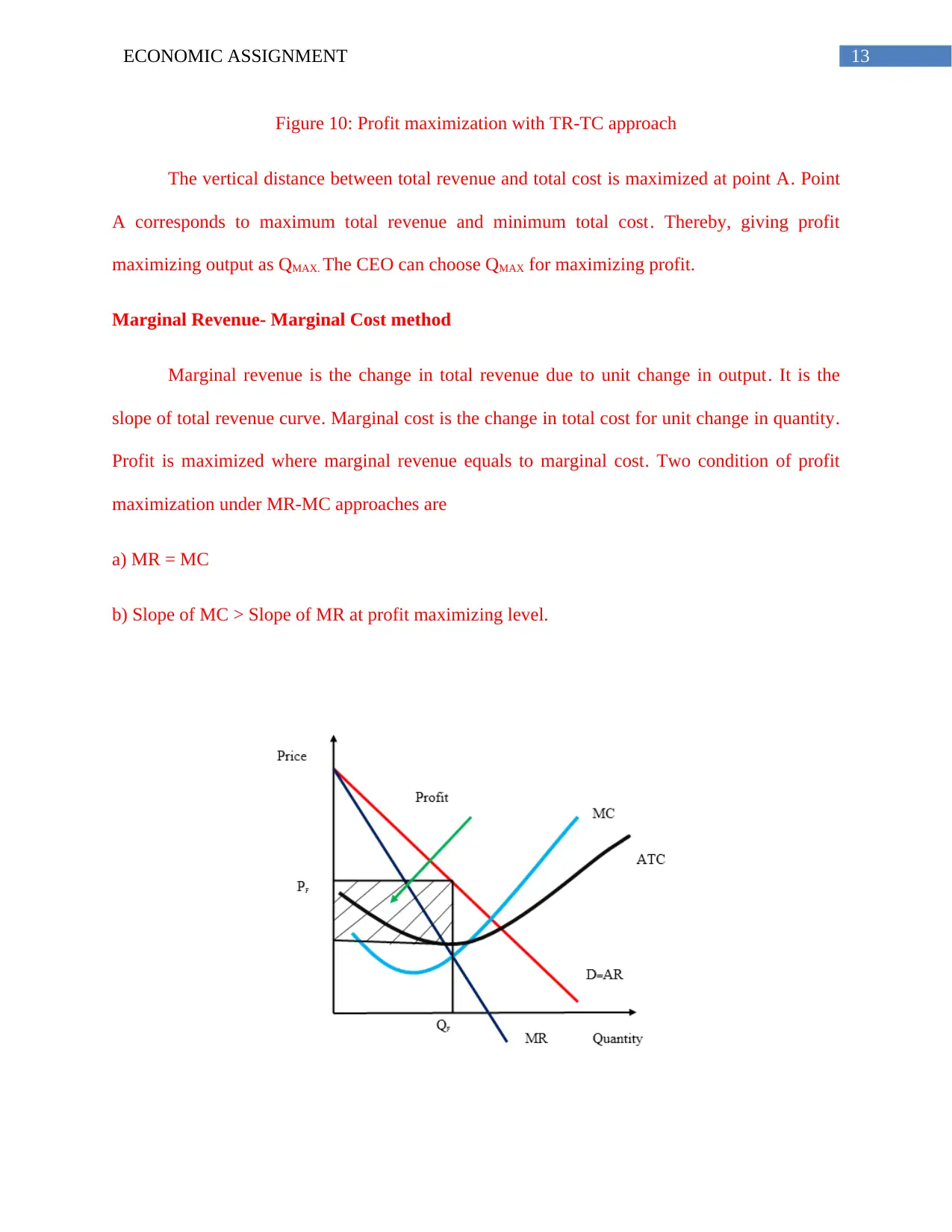
Marginal revenue is the change in total revenue due to unit change in output. It is the
slope of total revenue curve. Marginal cost is the change in total cost for unit change in quantity.
Profit is maximized where marginal revenue equals to marginal cost. Two condition of profit
maximization under MR-MC approaches are
a) MR = MC
b) Slope of MC > Slope of MR at profit maximizing level.
14ECONOMIC ASSIGNMENT
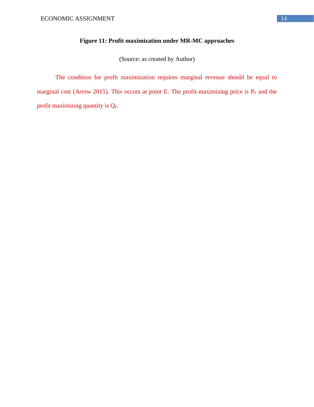
Figure 11: Profit maximization under MR-MC approaches
(Source: as created by Author)
The condition for profit maximization requires marginal revenue should be equal to
marginal cost (Arrow 2015). This occurs at point E. The profit-maximizing price is PF and the
profit maximizing quantity is QF.
Figure 11: Profit maximization under MR-MC approaches
(Source: as created by Author)
The condition for profit maximization requires marginal revenue should be equal to
marginal cost (Arrow 2015). This occurs at point E. The profit-maximizing price is PF and the
profit maximizing quantity is QF.
15ECONOMIC ASSIGNMENT
References
Arrow, K., 2015. Microeconomics and operations research: Their interactions and
differences. Information Systems Frontiers, 17(1), pp.3-9.
Cowen, T. and Tabarrok, A., 2015. Modern Principles of Microeconomics. Palgrave Macmillan.
Elsner, W., Heinrich, T. and Schwardt, H., 2014. The microeconomics of complex economies:
Evolutionary, institutional, neoclassical, and complexity perspectives. Academic Press.
Fine, B., 2016. Microeconomics. University of Chicago Press Economics Books.
Frank, R., 2014. Microeconomics and behavior. McGraw-Hill Higher Education.
McKenzie, R.B. and Lee, D.R., 2016. Microeconomics for MBAs: The economic way of thinking
for managers. Cambridge University Press.
Moulin, H., 2014. Cooperative microeconomics: a game-theoretic introduction. Princeton
University Press.
Nicholson, W. and Snyder, C.M., 2014. Intermediate microeconomics and its application.
Cengage Learning.
1 out of 16
Related Documents
Your All-in-One AI-Powered Toolkit for Academic Success.
+13062052269
info@desklib.com
Available 24*7 on WhatsApp / Email
![[object Object]](/_next/static/media/star-bottom.7253800d.svg)
Unlock your academic potential
© 2024 | Zucol Services PVT LTD | All rights reserved.


