MAT9004 Practice Exam Assignment PDF
Added on 2021-05-30
8 Pages859 Words85 Views
MAT9004 Practice Exam
MAT9004 Practice Exam
Institution Name
Student Name
Date
MAT9004 Practice Exam
Institution Name
Student Name
Date

MAT9004 Practice Exam
1. f ( x )=−2 x3−9 x2−12 x+ 2
a. f 1 ( x) is the derivative of f (x) with respect to x
using thepower rule, subtraction and additional rule we obtain
f 1 ( x ) =−6 x2−18 x−12
For x ∈ [−2,3]
b. f 1 ( x ) =−6 x2−18 x−12
f 11(x ) is the derivative of f 1 ( x ) with respect to x
Using the power rule, addition and the subtraction rule we obtain
f 11 ( x )=−12 x
Since x ∈ [−2,3] then
f 11 ( x )=−12 x for x ∈ [−2,3]
c. The stationery points are at point f 1 ( x )=0
Hence the stationery points will be at the roots of −6 x2−18 x−12
Using the quadratic equation x=−b ± √ b2−4 ac
2 a
We obtain the roots of the function at the points x=−1∧−2
The value of f ( x ) at the stationery points will be
f ( −1 ) =7∧f ( −2 ) =6
d. Finding local minimum and local maximum
The stationery points are at ( −1,7 ) ∧(−2,6)
Now we use the sign test to determine if the points are maximum
or minimum
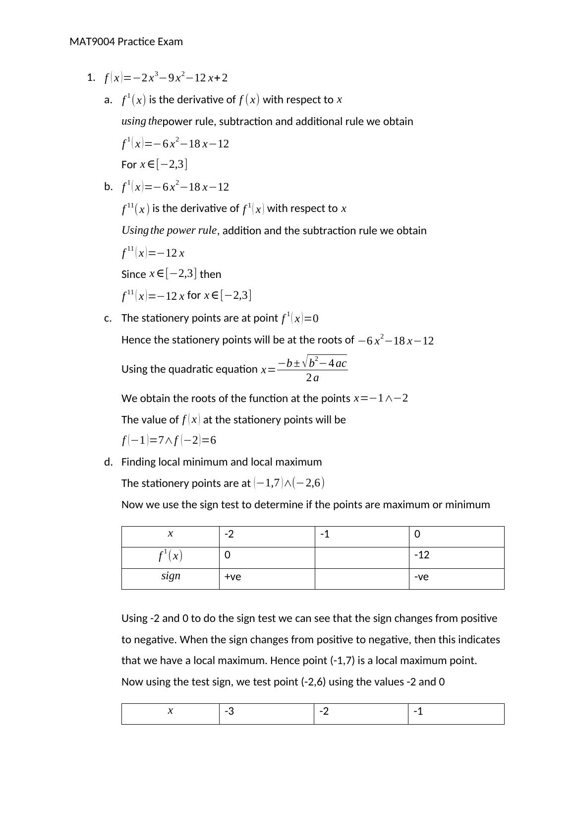
x -2 -1 0
f 1 ( x) 0 -12
sign +ve -ve
Using -2 and 0 to do the sign test we can see that the sign
changes from positive to negative. When the sign changes from
positive to negative, then this indicates that we have a local
maximum. Hence point (-1,7) is a local maximum point.
Now using the test sign, we test point (-2,6) using the values -2
and 0
1. f ( x )=−2 x3−9 x2−12 x+ 2
a. f 1 ( x) is the derivative of f (x) with respect to x
using thepower rule, subtraction and additional rule we obtain
f 1 ( x ) =−6 x2−18 x−12
For x ∈ [−2,3]
b. f 1 ( x ) =−6 x2−18 x−12
f 11(x ) is the derivative of f 1 ( x ) with respect to x
Using the power rule, addition and the subtraction rule we obtain
f 11 ( x )=−12 x
Since x ∈ [−2,3] then
f 11 ( x )=−12 x for x ∈ [−2,3]
c. The stationery points are at point f 1 ( x )=0
Hence the stationery points will be at the roots of −6 x2−18 x−12
Using the quadratic equation x=−b ± √ b2−4 ac
2 a
We obtain the roots of the function at the points x=−1∧−2
The value of f ( x ) at the stationery points will be
f ( −1 ) =7∧f ( −2 ) =6
d. Finding local minimum and local maximum
The stationery points are at ( −1,7 ) ∧(−2,6)
Now we use the sign test to determine if the points are maximum
or minimum
x -2 -1 0
f 1 ( x) 0 -12
sign +ve -ve
Using -2 and 0 to do the sign test we can see that the sign
changes from positive to negative. When the sign changes from
positive to negative, then this indicates that we have a local
maximum. Hence point (-1,7) is a local maximum point.
Now using the test sign, we test point (-2,6) using the values -2
and 0
MAT9004 Practice Exam
x -3 -2 -1
f 1 ( x) -2 0
sign -ve +ve
The sign is changing from negative to positive hence the point (-
2,6) is a local minimum.
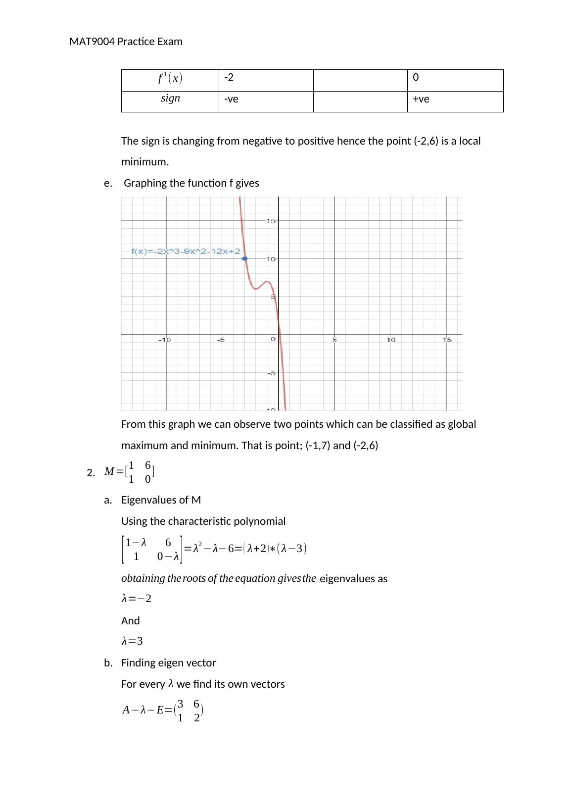
e. Graphing the function f gives
From this graph we can observe two points which can be
classified as global maximum and minimum. That is point; (-1,7)
and (-2,6)
2. M =[1 6
1 0]
a. Eigenvalues of M
Using the characteristic polynomial
[ 1−λ 6
1 0−λ ] =λ2 −λ−6= ( λ+2 )∗(λ−3)
obtaining the roots of the equation givesthe eigenvalues as
λ=−2
And
λ=3
b. Finding eigen vector
For every λ we find its own vectors
x -3 -2 -1
f 1 ( x) -2 0
sign -ve +ve
The sign is changing from negative to positive hence the point (-
2,6) is a local minimum.
e. Graphing the function f gives
From this graph we can observe two points which can be
classified as global maximum and minimum. That is point; (-1,7)
and (-2,6)
2. M =[1 6
1 0]
a. Eigenvalues of M
Using the characteristic polynomial
[ 1−λ 6
1 0−λ ] =λ2 −λ−6= ( λ+2 )∗(λ−3)
obtaining the roots of the equation givesthe eigenvalues as
λ=−2
And
λ=3
b. Finding eigen vector
For every λ we find its own vectors
End of preview
Want to access all the pages? Upload your documents or become a member.