Practical Statistics Assignment 4 for MATH 1P98: Detailed Solutions
VerifiedAdded on 2020/04/15
|15
|1313
|386
Homework Assignment
AI Summary
This document presents a detailed solution for Assignment 4 in MATH 1P98, a practical statistics course. The assignment covers various statistical concepts including confidence intervals (93% and 95%), hypothesis testing using Z-tests and t-tests, and chi-square tests. The solution addresses several questions involving different scenarios, such as analyzing the average attractiveness rating of men, testing claims about marathon completion rates, comparing evaluation ratings of male and female professors, and examining the difference in heights between presidents and their opponents. The assignment also includes an analysis of police call frequencies across different days of the week. Each question includes the formulation of hypotheses, computation of test statistics, determination of p-values, and conclusions based on the significance levels and confidence intervals. The solutions demonstrate the application of statistical techniques to real-world problems, providing insights and interpretations for each scenario.
MATH 1P98: PRACTICAL STATISTICS
ASSIGNMENT 4
STUDENT ID
[Pick the date]
ASSIGNMENT 4
STUDENT ID
[Pick the date]
Paraphrase This Document
Need a fresh take? Get an instant paraphrase of this document with our AI Paraphraser
Question 1
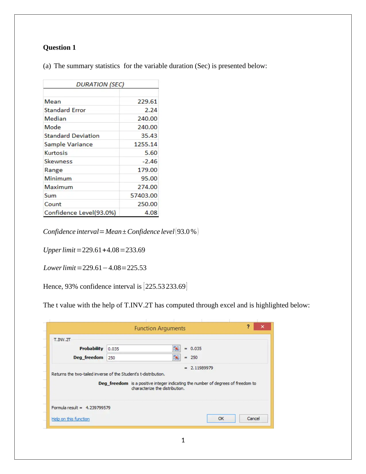
(a) The summary statistics for the variable duration (Sec) is presented below:
Confidence interval=Mean± Confidence level ( 93.0 % )
Upper limit =229.61+4.08=233.69
Lower limit =229.61−4.08=225.53
Hence, 93% confidence interval is [ 225.53 233.69 ]
The t value with the help of T.INV.2T has computed through excel and is highlighted below:
1
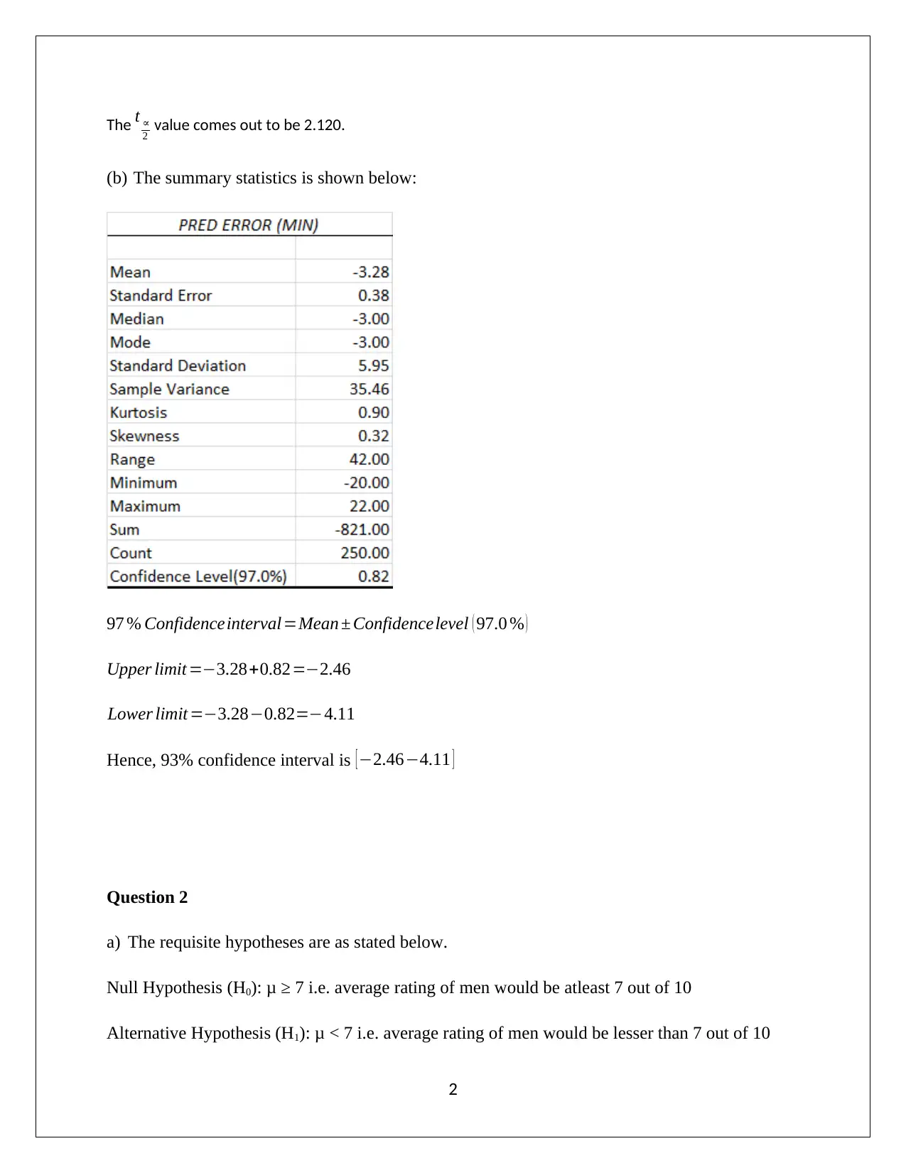
The t ∝
2 value comes out to be 2.120.
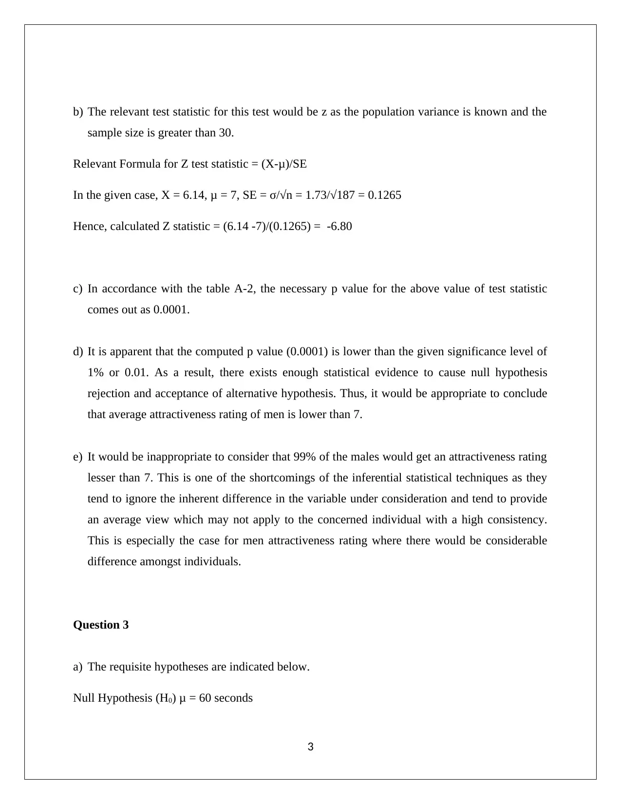
(b) The summary statistics is shown below:
97 % Confidenceinterval=Mean ± Confidencelevel ( 97.0 % )
Upper limit =−3.28+0.82=−2.46
Lower limit =−3.28−0.82=−4.11
Hence, 93% confidence interval is [−2.46−4.11 ]
Question 2
a) The requisite hypotheses are as stated below.
Null Hypothesis (H0): μ ≥ 7 i.e. average rating of men would be atleast 7 out of 10
Alternative Hypothesis (H1): μ < 7 i.e. average rating of men would be lesser than 7 out of 10
2
⊘ This is a preview!⊘
Do you want full access?
Subscribe today to unlock all pages.

Trusted by 1+ million students worldwide
b) The relevant test statistic for this test would be z as the population variance is known and the
sample size is greater than 30.
Relevant Formula for Z test statistic = (X-μ)/SE
In the given case, X = 6.14, μ = 7, SE = σ/√n = 1.73/√187 = 0.1265
Hence, calculated Z statistic = (6.14 -7)/(0.1265) = -6.80
c) In accordance with the table A-2, the necessary p value for the above value of test statistic
comes out as 0.0001.
d) It is apparent that the computed p value (0.0001) is lower than the given significance level of
1% or 0.01. As a result, there exists enough statistical evidence to cause null hypothesis
rejection and acceptance of alternative hypothesis. Thus, it would be appropriate to conclude
that average attractiveness rating of men is lower than 7.
e) It would be inappropriate to consider that 99% of the males would get an attractiveness rating
lesser than 7. This is one of the shortcomings of the inferential statistical techniques as they
tend to ignore the inherent difference in the variable under consideration and tend to provide
an average view which may not apply to the concerned individual with a high consistency.
This is especially the case for men attractiveness rating where there would be considerable
difference amongst individuals.
Question 3
a) The requisite hypotheses are indicated below.
Null Hypothesis (H0) μ = 60 seconds
3
Paraphrase This Document
Need a fresh take? Get an instant paraphrase of this document with our AI Paraphraser
Alternative Hypothesis (H1): μ ≠ 60 seconds
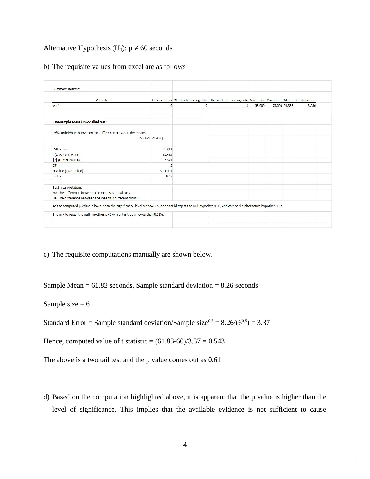
b) The requisite values from excel are as follows
c) The requisite computations manually are shown below.
Sample Mean = 61.83 seconds, Sample standard deviation = 8.26 seconds
Sample size = 6
Standard Error = Sample standard deviation/Sample size0.5 = 8.26/(60.5) = 3.37
Hence, computed value of t statistic = (61.83-60)/3.37 = 0.543
The above is a two tail test and the p value comes out as 0.61
d) Based on the computation highlighted above, it is apparent that the p value is higher than the
level of significance. This implies that the available evidence is not sufficient to cause
4
rejection of null hypothesis. Hence, the alternative hypothesis would not be accepted.. Thus,
the original claim has been validated through hypothesis testing.
Question 4
Number of men finished marathon n1= 24,521
Number of men dropped out marathon x1= 283
Number of women finished marathon n2= 12,853
Number of women dropped out marathon x2= 152
Significance level = 0.05
(a) Hypotheses
Null hypothesis Ho : p1− p2=0
Alternative hypothesis H1 : p1−p2 ≠ 0
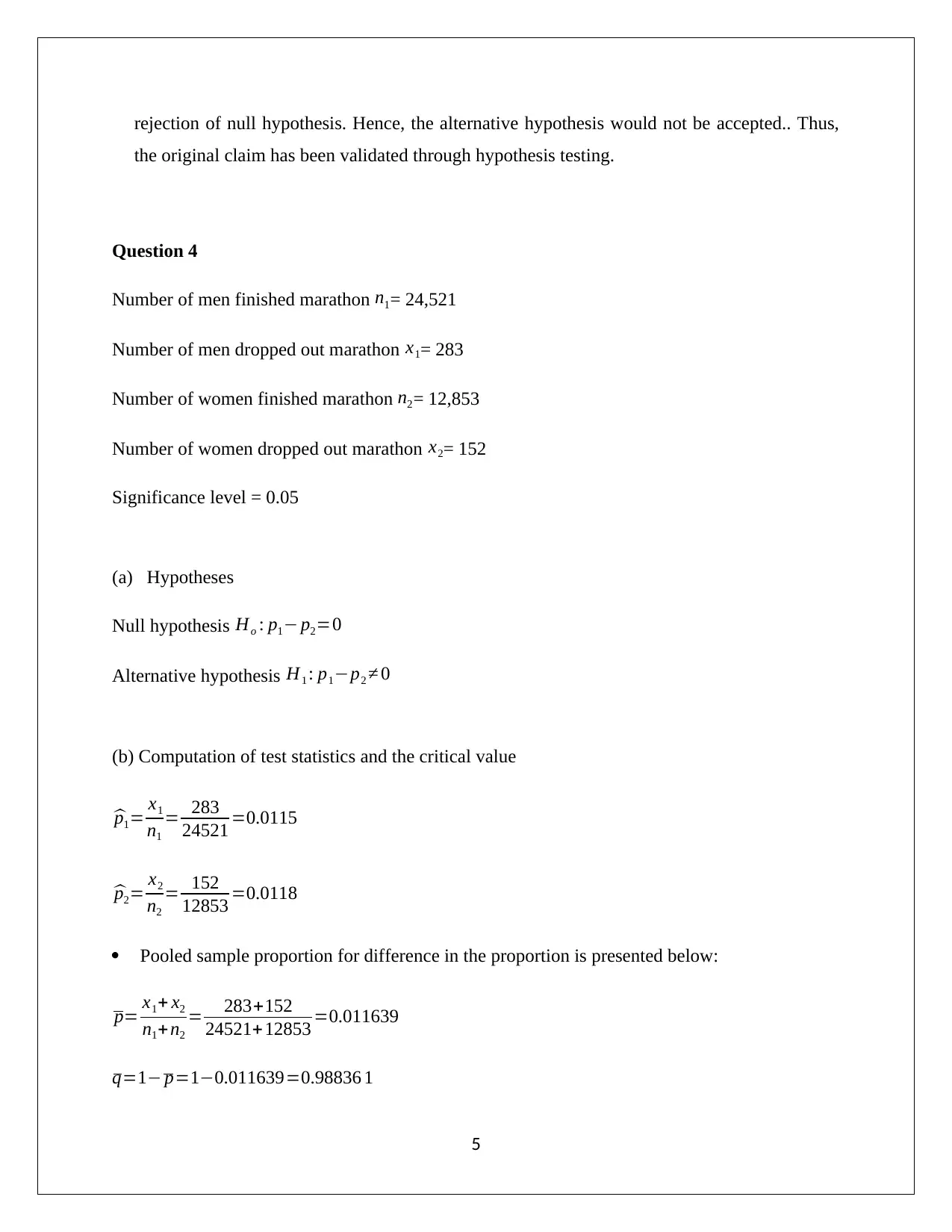
(b) Computation of test statistics and the critical value
^p1= x1
n1
= 283
24521 =0.0115
^p2= x2
n2
= 152
12853 =0.0118
Pooled sample proportion for difference in the proportion is presented below:
p= x1+ x2
n1+n2
= 283+152
24521+12853 =0.011639
q=1− p=1−0.011639=0.98836 1
5
⊘ This is a preview!⊘
Do you want full access?
Subscribe today to unlock all pages.

Trusted by 1+ million students worldwide
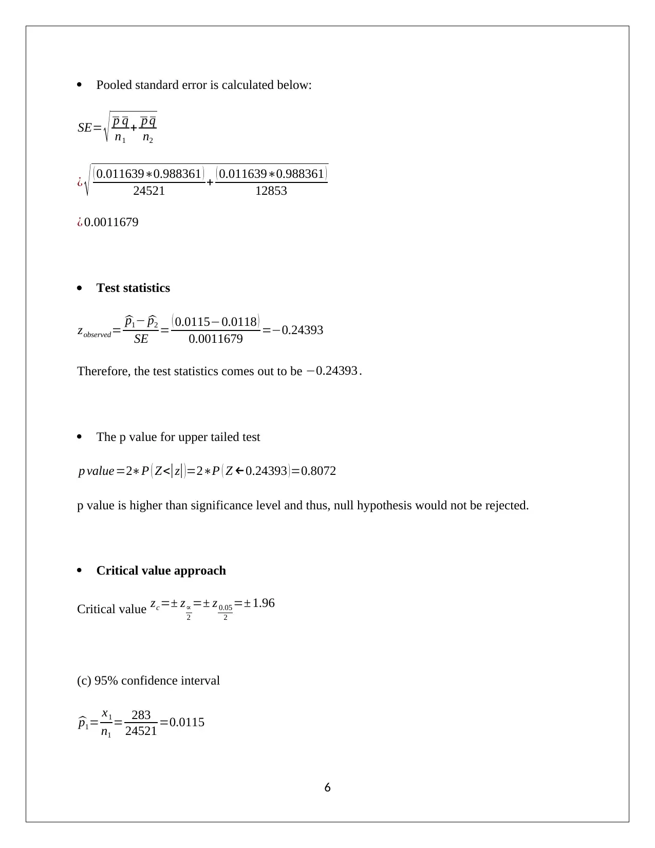
Pooled standard error is calculated below:
SE= √ p q
n1
+ p q
n2
¿ √ ( 0.011639∗0.988361 )
24521 + ( 0.011639∗0.988361 )
12853
¿ 0.0011679
Test statistics
zobserved= ^p1− ^p2
SE = ( 0.0115−0.0118 )
0.0011679 =−0.24393
Therefore, the test statistics comes out to be −0.24393 .
The p value for upper tailed test
p value=2∗P ( Z<| z|)=2∗P ( Z ←0.24393 ) =0.8072
p value is higher than significance level and thus, null hypothesis would not be rejected.
Critical value approach
Critical value zc=± z∝
2
=± z 0.05
2
=± 1.96
(c) 95% confidence interval
^p1= x1
n1
= 283
24521 =0.0115
6
Paraphrase This Document
Need a fresh take? Get an instant paraphrase of this document with our AI Paraphraser
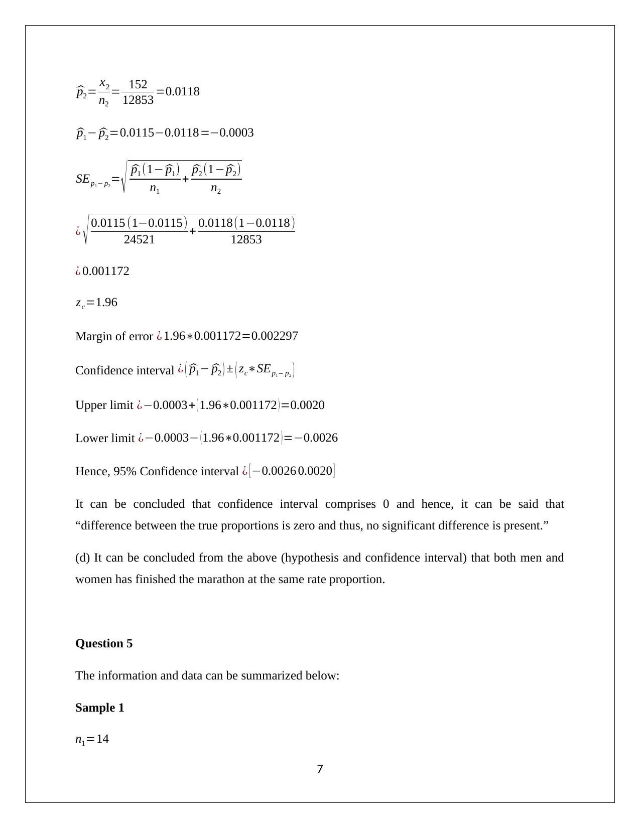
^p2= x2
n2
= 152
12853 =0.0118
^p1− ^p2=0.0115−0.0118=−0.0003
SEp1− p2
= √ ^p1 (1− ^p1)
n1
+ ^p2 (1− ^p2)
n2
¿ √ 0.0115 (1−0.0115)
24521 + 0.0118(1−0.0118)
12853
¿ 0.001172
zc=1.96
Margin of error ¿ 1.96∗0.001172=0.002297
Confidence interval ¿ ( ^p1− ^p2 ) ± ( zc∗SEp1 – p2 )
Upper limit ¿−0.0003+ ( 1.96∗0.001172 )=0.0020
Lower limit ¿−0.0003− (1.96∗0.001172 )=−0.0026
Hence, 95% Confidence interval ¿ [ −0.0026 0.0020 ]
It can be concluded that confidence interval comprises 0 and hence, it can be said that
“difference between the true proportions is zero and thus, no significant difference is present.”
(d) It can be concluded from the above (hypothesis and confidence interval) that both men and
women has finished the marathon at the same rate proportion.
Question 5
The information and data can be summarized below:
Sample 1
n1=14
7
n2
= 152
12853 =0.0118
^p1− ^p2=0.0115−0.0118=−0.0003
SEp1− p2
= √ ^p1 (1− ^p1)
n1
+ ^p2 (1− ^p2)
n2
¿ √ 0.0115 (1−0.0115)
24521 + 0.0118(1−0.0118)
12853
¿ 0.001172
zc=1.96
Margin of error ¿ 1.96∗0.001172=0.002297
Confidence interval ¿ ( ^p1− ^p2 ) ± ( zc∗SEp1 – p2 )
Upper limit ¿−0.0003+ ( 1.96∗0.001172 )=0.0020
Lower limit ¿−0.0003− (1.96∗0.001172 )=−0.0026
Hence, 95% Confidence interval ¿ [ −0.0026 0.0020 ]
It can be concluded that confidence interval comprises 0 and hence, it can be said that
“difference between the true proportions is zero and thus, no significant difference is present.”
(d) It can be concluded from the above (hypothesis and confidence interval) that both men and
women has finished the marathon at the same rate proportion.
Question 5
The information and data can be summarized below:
Sample 1
n1=14
7
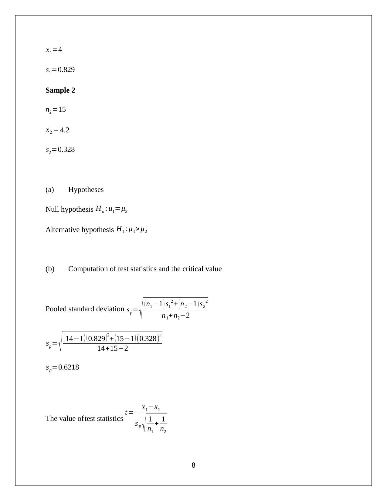
x1=4
s1=0.829
Sample 2
n2 =15
x2 = 4.2
s2=0.328
(a) Hypotheses
Null hypothesis Ho : μ1=μ2
Alternative hypothesis H1 : μ1> μ2
(b) Computation of test statistics and the critical value
Pooled standard deviation sp= √ ( n1 −1 ) s1
2 + ( n2−1 ) s2
2
n1+n2−2
sp= √ ( 14−1 ) ( 0.829 ) 2+ ( 15−1 ) (0.328)2
14+15−2
sp=0.6218
The value oftest statistics t= x1−x2
s p √ 1
n1
+ 1
n2
8
⊘ This is a preview!⊘
Do you want full access?
Subscribe today to unlock all pages.

Trusted by 1+ million students worldwide
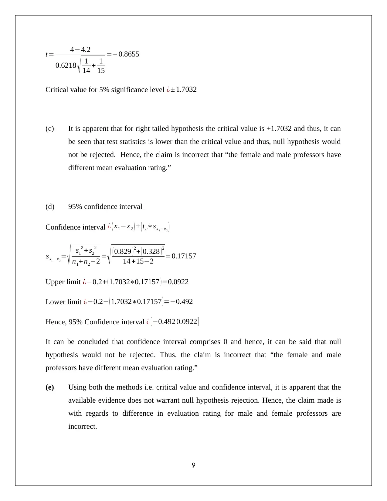
t= 4−4.2
0.6218 √ 1
14 + 1
15
=−0.8655
Critical value for 5% significance level ¿ ± 1.7032
(c) It is apparent that for right tailed hypothesis the critical value is +1.7032 and thus, it can
be seen that test statistics is lower than the critical value and thus, null hypothesis would
not be rejected. Hence, the claim is incorrect that “the female and male professors have
different mean evaluation rating.”
(d) 95% confidence interval
Confidence interval ¿ ( x1−x2 ) ± ( tc∗sx1−x2 )
sx1− x2
= √ s1
2 + s2
2
n1+n2−2 = √ ( 0.829 )2+ ( 0.328 )2
14 +15−2 =0.17157
Upper limit ¿−0.2+ ( 1.7032∗0.17157 ) =0.0922
Lower limit ¿−0.2− ( 1.7032∗0.17157 )=−0.492
Hence, 95% Confidence interval ¿ [ −0.492 0.0922 ]
It can be concluded that confidence interval comprises 0 and hence, it can be said that null
hypothesis would not be rejected. Thus, the claim is incorrect that “the female and male
professors have different mean evaluation rating.”
(e) Using both the methods i.e. critical value and confidence interval, it is apparent that the
available evidence does not warrant null hypothesis rejection. Hence, the claim made is
with regards to difference in evaluation rating for male and female professors are
incorrect.
9
Paraphrase This Document
Need a fresh take? Get an instant paraphrase of this document with our AI Paraphraser
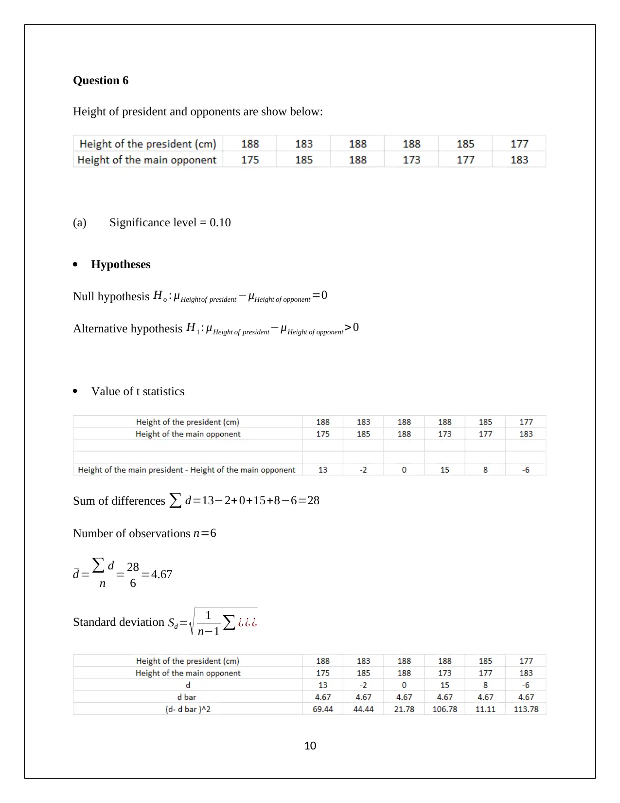
Question 6
Height of president and opponents are show below:
(a) Significance level = 0.10
Hypotheses
Null hypothesis Ho : μHeight of president −μHeight of opponent =0
Alternative hypothesis H1 : μHeight of president−μHeight of opponent > 0
Value of t statistics
Sum of differences ∑ d=13−2+ 0+15+8−6=28
Number of observations n=6
d =∑ d
n = 28
6 =4.67
Standard deviation Sd = √ 1
n−1 ∑ ¿ ¿ ¿
10
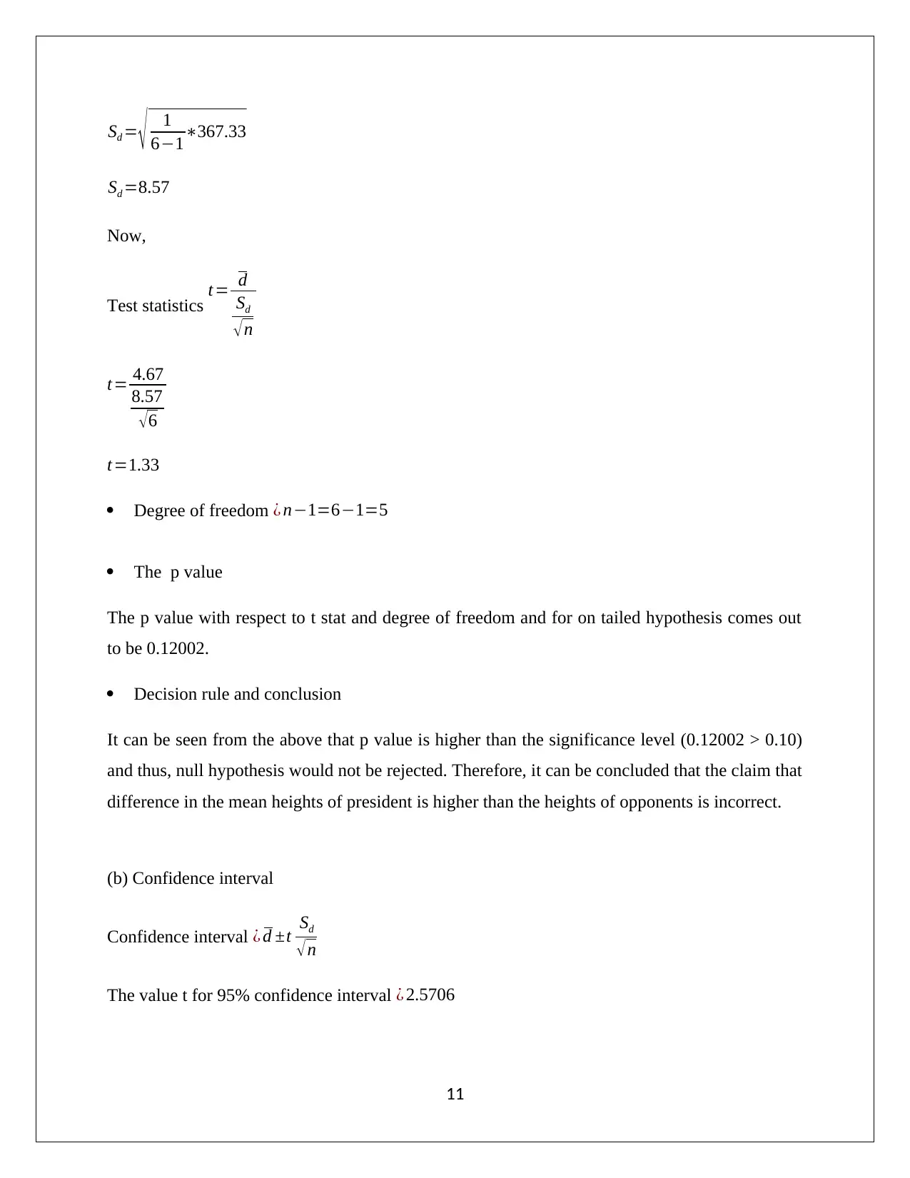
Sd = √ 1
6−1∗367.33
Sd =8.57
Now,
Test statistics t= d
Sd
√ n
t= 4.67
8.57
√ 6
t=1.33
Degree of freedom ¿ n−1=6−1=5
The p value
The p value with respect to t stat and degree of freedom and for on tailed hypothesis comes out
to be 0.12002.
Decision rule and conclusion
It can be seen from the above that p value is higher than the significance level (0.12002 > 0.10)
and thus, null hypothesis would not be rejected. Therefore, it can be concluded that the claim that
difference in the mean heights of president is higher than the heights of opponents is incorrect.
(b) Confidence interval
Confidence interval ¿ d ±t Sd
√n
The value t for 95% confidence interval ¿ 2.5706
11
⊘ This is a preview!⊘
Do you want full access?
Subscribe today to unlock all pages.

Trusted by 1+ million students worldwide
1 out of 15
Related Documents
Your All-in-One AI-Powered Toolkit for Academic Success.
+13062052269
info@desklib.com
Available 24*7 on WhatsApp / Email
![[object Object]](/_next/static/media/star-bottom.7253800d.svg)
Unlock your academic potential
Copyright © 2020–2026 A2Z Services. All Rights Reserved. Developed and managed by ZUCOL.

![Statistics Assignment: Hypothesis Testing Solutions - [University]](/_next/image/?url=https%3A%2F%2Fdesklib.com%2Fmedia%2Fimages%2Fbj%2F2a126809566149e6af44fcc81b2e9526.jpg&w=256&q=75)


