Equilibrium Prices in a Two-Sector Economy

This assignment focuses on determining the equilibrium prices of goods and services in a two-sector economy. It utilizes Polya's four-step problem-solving method, constructing an exchange table to represent the flow of outputs between sectors. The assignment then employs matrix algebra techniques, including row reduction of an augmented matrix, to solve for the equilibrium prices. The final solution demonstrates the concept of price ratios and how they remain constant despite proportionate price changes.

Running head: APPLIED LINEAR ALGEBRA 1
Applied Linear Algebra
Name
Institution
1

APPLIED LINEAR ALGEBRA 2
Applied Linear Algebra
Question 1
According to Polya, four step-by-step techniques are used to solve any problem. First,
understand the problem.
Evidently, the problem requires the equilibrium prices of two sectors (goods and services) that
can make expenditures equivalent to expenses. In the question, Goods sell 80% worth of its
outputs to the services economy. On the other hand, Services sell 70% worth of outputs to Goods
sector.
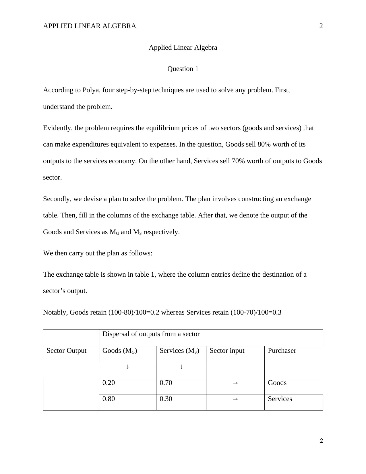
Secondly, we devise a plan to solve the problem. The plan involves constructing an exchange
table. Then, fill in the columns of the exchange table. After that, we denote the output of the
Goods and Services as MG and MS respectively.
We then carry out the plan as follows:
The exchange table is shown in table 1, where the column entries define the destination of a
sector’s output.
Notably, Goods retain (100-80)/100=0.2 whereas Services retain (100-70)/100=0.3
Dispersal of outputs from a sector
Sector Output Goods (MG) Services (MS) Sector input Purchaser
↓ ↓
0.20 0.70 → Goods
0.80 0.30 → Services
2

APPLIED LINEAR ALGEBRA 3
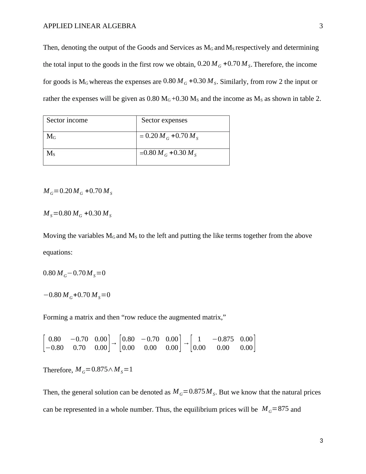
Then, denoting the output of the Goods and Services as MG and MS respectively and determining
the total input to the goods in the first row we obtain, 0.20 M G +0.70 M S. Therefore, the income
for goods is MG whereas the expenses are 0.80 M G +0.30 MS. Similarly, from row 2 the input or
rather the expenses will be given as 0.80 MG +0.30 MS and the income as MS as shown in table 2.
Sector income Sector expenses
MG = 0.20 M G +0.70 M S
MS =0.80 M G +0.30 M S
M G=0.20 M G +0.70 M S
M S =0.80 MG +0.30 M S
Moving the variables MG and MS to the left and putting the like terms together from the above
equations:
0.80 MG−0.70 M S =0
−0.80 MG +0.70 MS =0
Forming a matrix and then “row reduce the augmented matrix,”
[ 0.80 −0.70 0.00
−0.80 0.70 0.00 ] → [ 0.80 −0.70 0.00
0.00 0.00 0.00 ] → [ 1 −0.875 0.00
0.00 0.00 0.00 ]
Therefore, M G=0.875∧M S =1
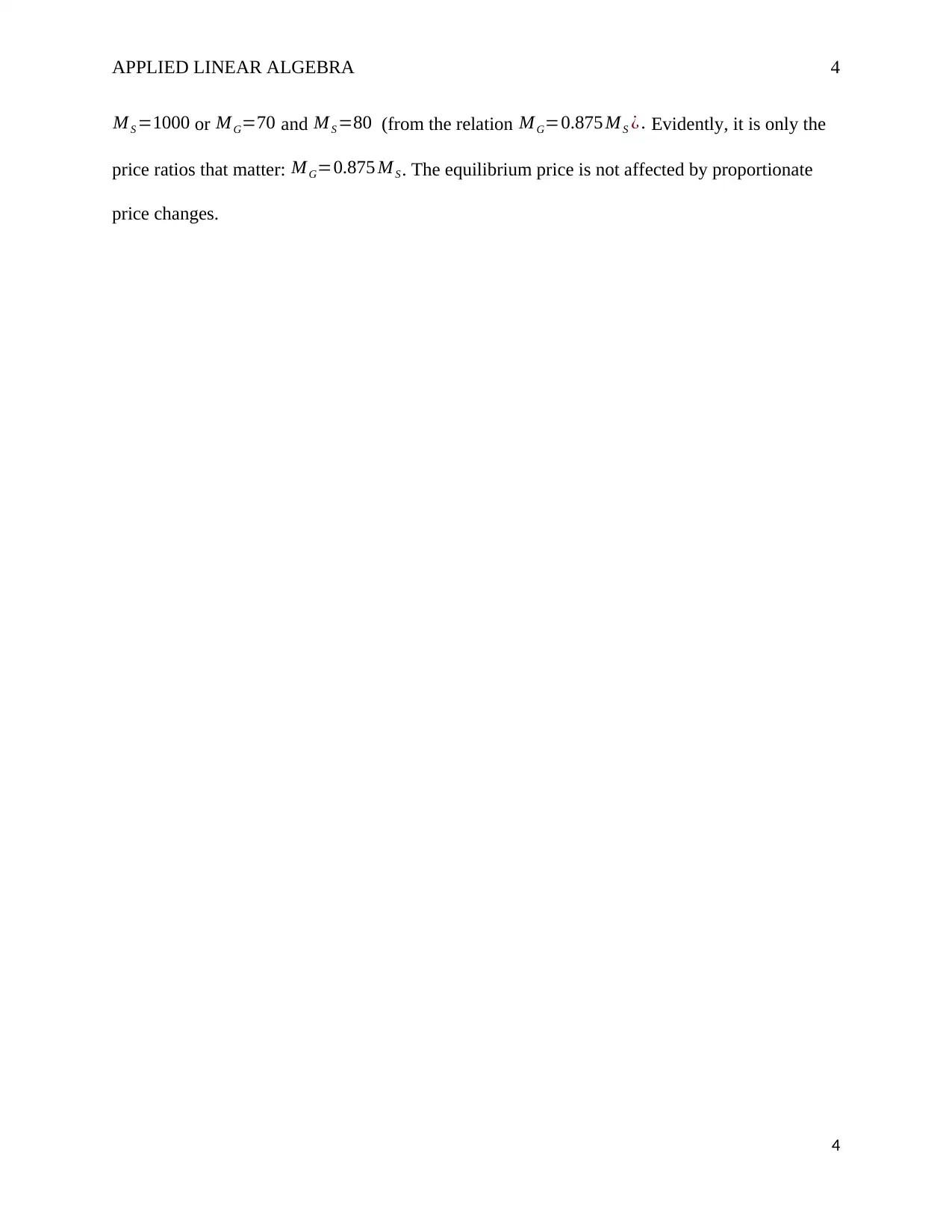
Then, the general solution can be denoted as M G=0.875 MS. But we know that the natural prices
can be represented in a whole number. Thus, the equilibrium prices will be M G=875 and
3

APPLIED LINEAR ALGEBRA 4
M S =1000 or M G=70 and M S =80 (from the relation M G=0.875 M S ¿ . Evidently, it is only the
price ratios that matter: M G=0.875 M S . The equilibrium price is not affected by proportionate
price changes.
4