Math Homework - Desklib

This study material on math homework covers topics such as quadratic functions, regression, and models. It explains how to model tables and graphs using quadratic functions and regression. It also covers finding the vertex form of quadratic equations and solving real-life problems using quadratic models. The content includes solved examples and diagrams. The subject is math, and the course code and college/university are not mentioned.

Running head: MATH HOMEWORK 1
Math Homework
Name
Institution

MATH HOMEWORK 2
Math Homework
Question 1
A quadratic function has a series of varying positive gradients on one part and a series of varying
negative gradients on the other part. The positive and negative gradients meet at a point where
the gradient is zero hence forming a maximum point or a minimum point. The model in part C
has a negative gradient in the range −4 ≤ x ≤0. That is,
0−3
−2−−4 =−1.5 ,∧−1−0
0−−2 =−0.5
Additionally, the model has a series of varying positive gradients in the range 2 ≤ x ≤14.
3−0
4−2 =1.5 , 8−3
6−4 =2.5 , 15−8
8−6 =3.5 … 48−35
14−12 =6. 5
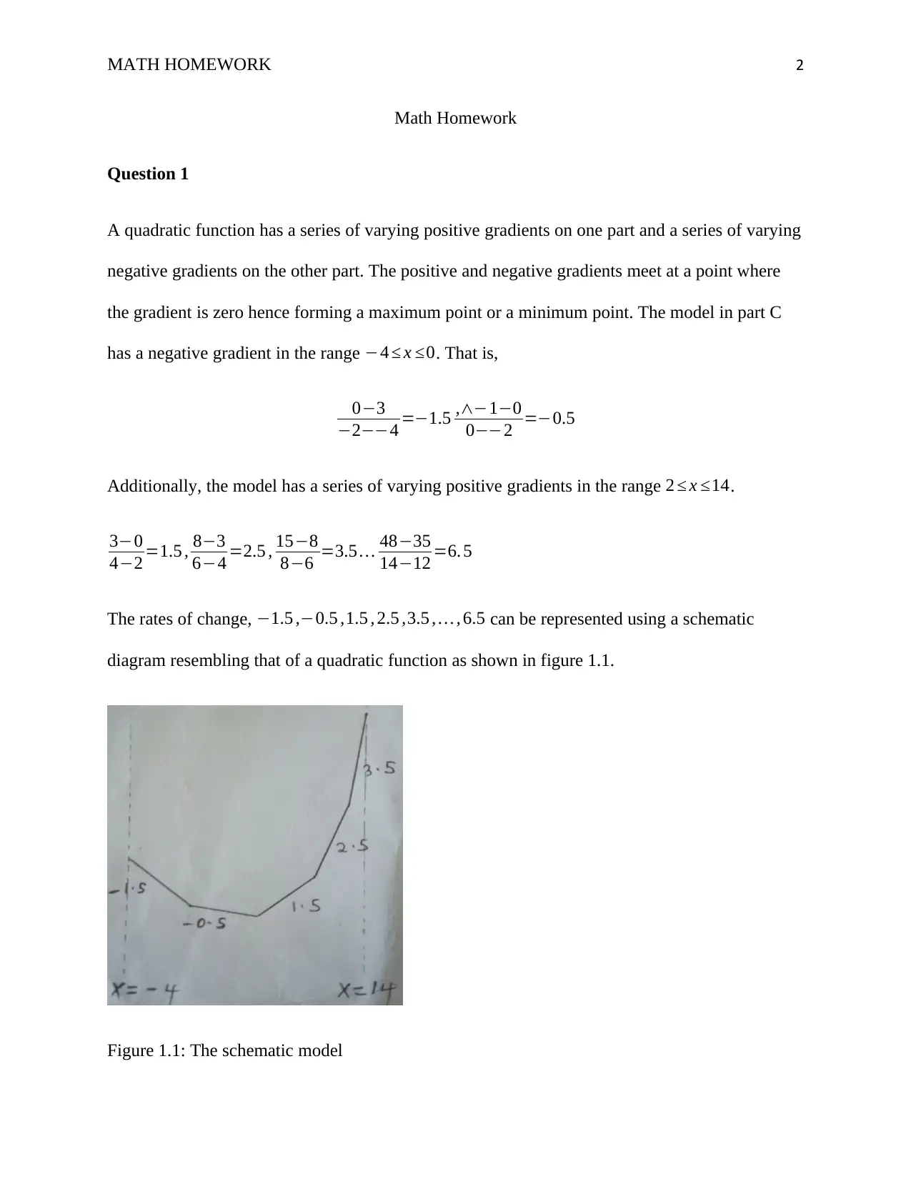
The rates of change, −1.5 ,−0.5 ,1.5 , 2.5 ,3.5 , … , 6.5 can be represented using a schematic
diagram resembling that of a quadratic function as shown in figure 1.1.
Figure 1.1: The schematic model

MATH HOMEWORK 3
Therefore, table C can be modelled as a quadratic function.
Question 2
part a
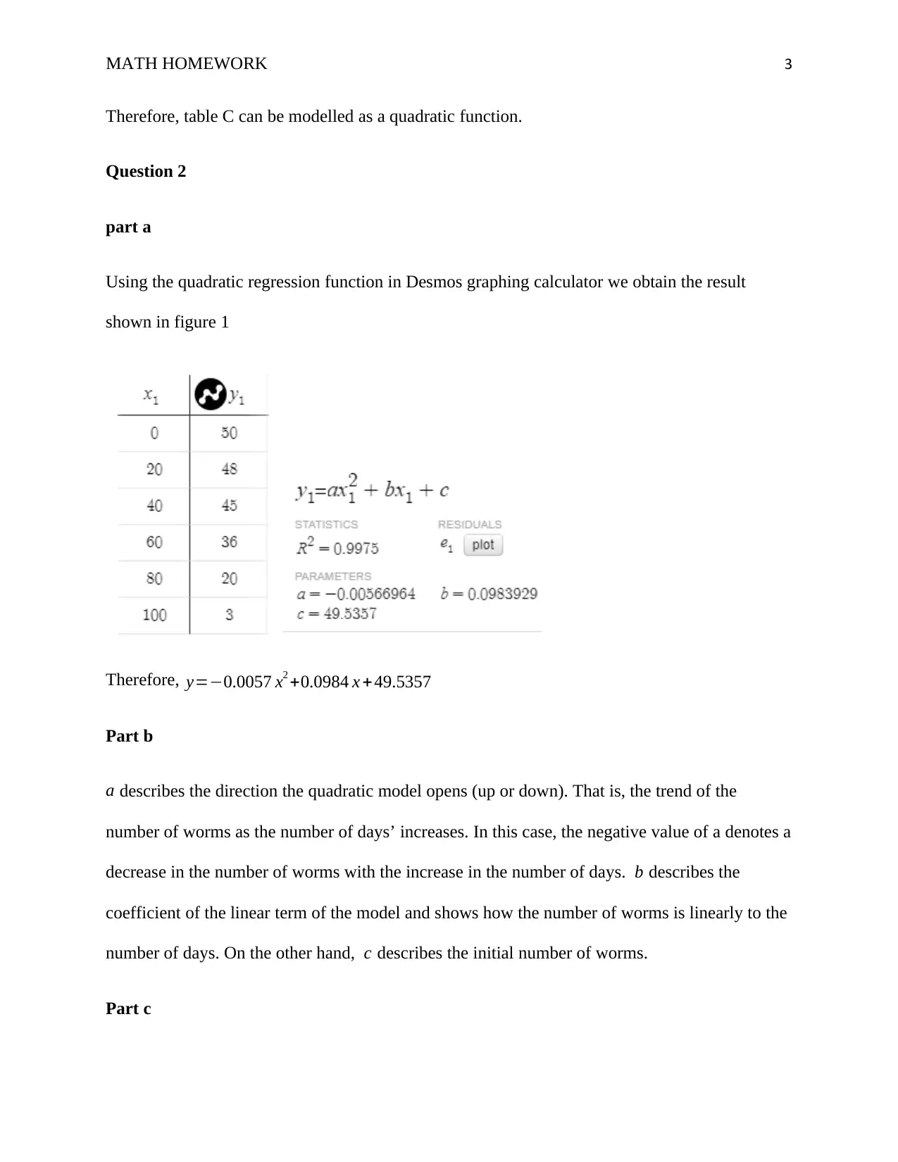
Using the quadratic regression function in Desmos graphing calculator we obtain the result
shown in figure 1
Therefore, y=−0.0057 x2 +0.0984 x +49.5357
Part b
a describes the direction the quadratic model opens (up or down). That is, the trend of the
number of worms as the number of days’ increases. In this case, the negative value of a denotes a
decrease in the number of worms with the increase in the number of days. b describes the
coefficient of the linear term of the model and shows how the number of worms is linearly to the
number of days. On the other hand, c describes the initial number of worms.
Part c

MATH HOMEWORK 4
y=0 ( when all worms die ) . That is , y=−0.0057 x2+ 0.0984 x+ 49.5357=0
Solving for x using the quadratic formula,
x=−b
2 a ± √b2−4 ac
2 a = −0.0984
−2(0.0057) ± √0.09842−4 (−0.0057)(49.5357)
−2(0.0057)
x=8.6316 ± 93.6215 , x=102.2531days∨x =−84.9899 days
We ignore x=−84.9899 days since the number of days can’t be negative.
Hence, it takes 102.2531 days for all the worms to die.
Question 3
Part a
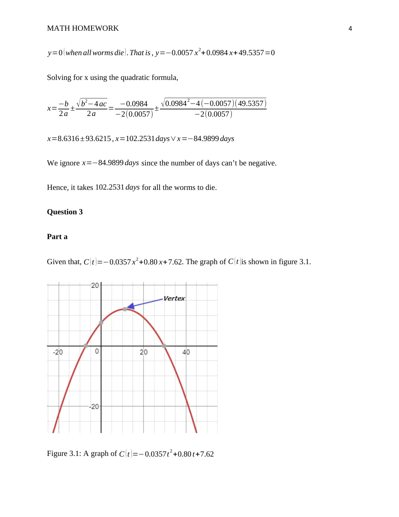
Given that, C ( t ) =−0.0357 x2 +0.80 x+7.62. The graph of C ( t )is shown in figure 3.1.
Figure 3.1: A graph of C ( t )=−0.0357t2 +0.80 t+7.62

MATH HOMEWORK 5
At the vertex, dC ( t )
dt =0
dC ( t )
dt =−0.0357 ( 2 ) t+0.80=0
0.0357 ( 2 ) t=0.80=0 ,t= 0.80
0.0357 ×2 =11.20
When t=11.20 , C ( t ) =−0.0357 ( 11.2 ) 2 +0.80 ( 11.20 ) +7.62=12.10
Hence, the vertex is (11.20 , 12.10)
Part b
The vertex form of the equation C ( t )=−0.0357t2 +0.80 t+7.62 is in the form C ( t )=a(t−h)2 +k
where h , k is the vertex.
But we know that, a=−0.0357 , h=11.20 , k=12.10
C ( t )=a(t−h)2 +k=−0.0357 ( t−11.20 )2 +12.10
Therefore, the vertex form is, C ( t )=−0.0357 ( t−11.20 )2+12.10
Part c
C ( t )=−0.0357t2 +0.80 t+7.6 2
The years when C ( t )=10 million
We substitute 10 into the quadratic model and solve for t using the quadratic formula.
C ( t )=−0.0357t2 +0.80 t+7.6 2=10

MATH HOMEWORK 6
−0.0357 t 2+0.80 t+7.6 2−10=0
−0.0357 t2+ 0.80 t−2.38=0
a=−0.0357 , b=0.80 , c=−2.38
t=−b
2 a ± √ b2−4 ac
2 a = −0.80
2(−0.0357) ± √0.802−4 (−0.0357)(−2.38)
2 (−0.0357)
t=11.2045 ±7.6729 , t=18.8774 years∨t=3.5316 years
The number of crimes committed was equal to 10million in the years (3.5316+1980) and
(1980+18.8774). That is, 1983.5316 and 1998.8774.
That is, approximately during the years 1983 and 1998.
Question 4
Part a
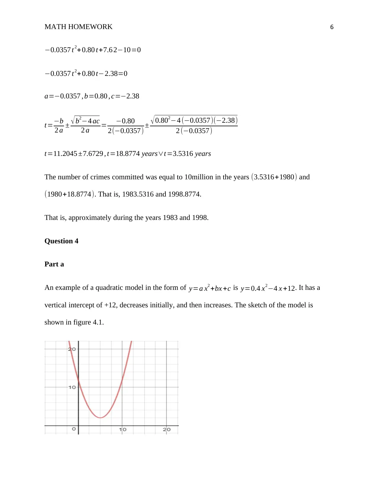
An example of a quadratic model in the form of y=a x2 +bx +c is y=0.4 x2−4 x +12. It has a
vertical intercept of +12, decreases initially, and then increases. The sketch of the model is
shown in figure 4.1.

MATH HOMEWORK 7
Figure 4.1: A graph of the model, y=0.4 x2−4 x +12
Part b
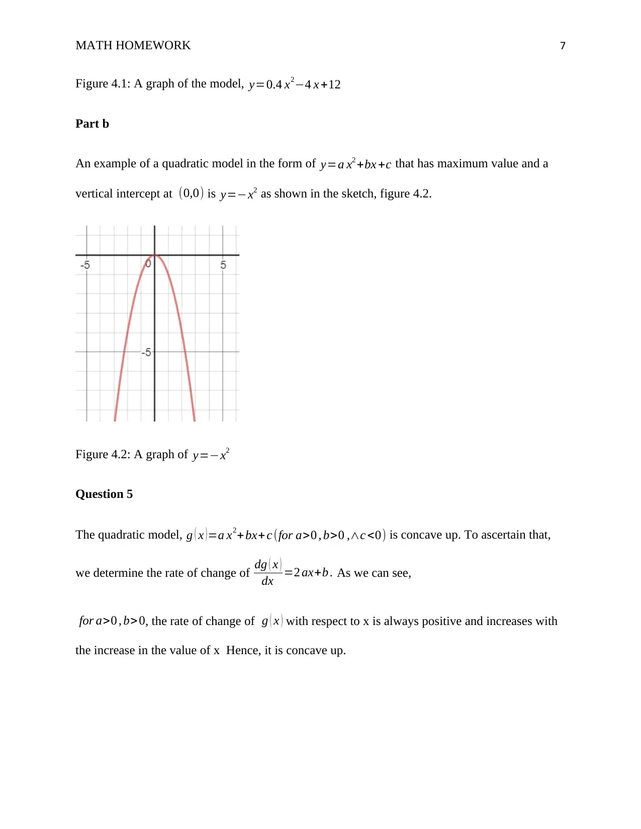
An example of a quadratic model in the form of y=a x2 +bx +c that has maximum value and a
vertical intercept at (0,0) is y=−x2 as shown in the sketch, figure 4.2.
Figure 4.2: A graph of y=−x2
Question 5
The quadratic model, g ( x )=a x2+ bx+ c (for a>0 , b>0 ,∧c <0) is concave up. To ascertain that,
we determine the rate of change of dg ( x )
dx =2 ax+b . As we can see,
for a>0 , b>0, the rate of change of g ( x ) with respect to x is always positive and increases with
the increase in the value of x Hence, it is concave up.