Mathematics for Construction

This document provides study material for Mathematics for Construction. It includes solved assignments, essays, and dissertations related to various topics in the subject. The document covers scenarios and equations related to length, width, velocity, power, lift, geometric progression, logarithms, and more.

Mathematics for Construction
1

Contents
Contents...........................................................................................................................................2
TASK 1............................................................................................................................................3
Scenario 1........................................................................................................................................3
1...................................................................................................................................................3
2...................................................................................................................................................3
Scenario 2........................................................................................................................................4
Scenario 3........................................................................................................................................5
1...................................................................................................................................................5
2...................................................................................................................................................6
3...................................................................................................................................................7
TASK 2............................................................................................................................................8
Scenario 1........................................................................................................................................8
(a).................................................................................................................................................8
(b).................................................................................................................................................8
(c)...............................................................................................................................................10
Scenario 2......................................................................................................................................12
TASK 3..........................................................................................................................................12
Scenario 1......................................................................................................................................12
Scenario 2......................................................................................................................................14
TASK 4..........................................................................................................................................15
Scenario 1..................................................................................................................................15
Scenario 2..................................................................................................................................18
Scenario 3..................................................................................................................................19
2

TASK 1
Scenario 1
1.
Let x be the length, then:
l * w = 26.5
thus,
x * (x-3.2) = 26.5
x2 – 3.2x = 26.5
x2 – 3.2x - 26.5 = 0
Solving quadratic equation applying quadratic yield formula:
x = {- (-3.2) +/- √ [(-3.2)2 – 4 * 1 * (- 26.5)]} / 2 * 1
x = 6.99 m
Length = 6.99 m
Width = 6.99 – 3.2 = 3.79 m
2.
If she is 5 days late she receives = £4250
if she is 12 days late she receives = £2120
Difference in amount she receives = £4250 - £2120 = £2130
Difference in days late = 12 days – 5 days = 7 days
Then per day pay is = £ 2130 / 7 = £ 304.28
So, constant pay is = 5771.4
Penalty per day is = 304.28
3

Scenario 2
A
i. Fd = 0.5 *  * u2 * Cd * A
Solution
Fd = Force thus its dimension is: [M1L1T-2]
Similarly, on Right hand side
 = density = kg / meter cube = [M1L-3T0]
A = meter square = [M0L2T0]
Cd = No dimension
u2 = velocity = u2 = [meter/ second]2 = [M0L2T-2]
0.5 *  * u2 * Cd * A = [M1L-3T0] * [M0L2T-2] * [M0L2T0]
= [M1L1T-2]
Thus LHS = RHS and equation can be said to be dimensionally correct.
ii) Power (P) = [M1L2T-3]
Weight (W) = [M1L-2T-2]
Height (h) = [M0L1T0]
Fluid flow rate (q) = [M0L3T-1]
Solution
Power is proportional to W; h and q thus :
Power = flow rate * work done
P = q * Work
Work = mass * height * gravity
Work = (Weight /G) * h * g
G and g can be considered as constant
Thus dimension of work = dimension of weight * dimension of height
dimension of work = [M1L-2T-2] * [M0L1T0]
Power = flow rate * work done
= [M0L3T-1] * [M1L-2T-2] * [M0L1T0]
4

Power = [M1L2T-3]
Hence dimensions are verified
Thus equation of power is:
P = q * (W /G) * h * g
Where
Q = fluid flow rate
w = weight
h = height
g = 9.8 m/s2
G = 6.67x10-11 (N-m2/kg2)
b. Lift = k*  * V2 * A
Solution
k= no dimension
 = kg / meter cube = [M1L-3T0]
A = meter square = [M0L2T0]
V2 = [meter/ second]2 = [M0L2T-2]
Lift = [M1L-3T0] * [M0L2T-2] * [M0L2T0]
Lift = [M1L1T-2]
Thus dimensions of lift are:(Kilogram*meter) per second square = Newton
Scenario 3
1.
(i) -2b/3
5

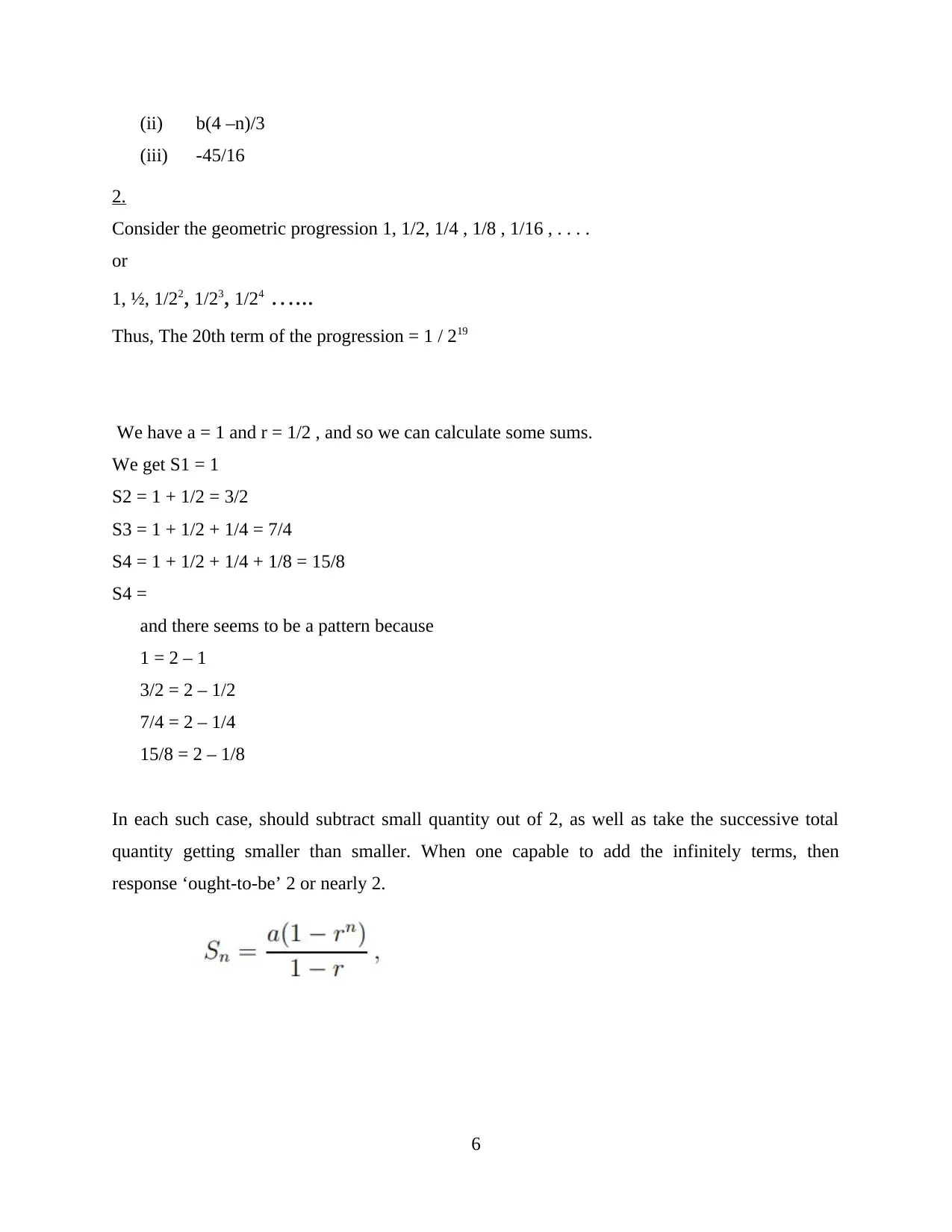
(ii) b(4 –n)/3
(iii) -45/16
2.
Consider the geometric progression 1, 1/2, 1/4 , 1/8 , 1/16 , . . . .
or
1, ½, 1/22, 1/23, 1/24 …...
Thus, The 20th term of the progression = 1 / 219
We have a = 1 and r = 1/2 , and so we can calculate some sums.
We get S1 = 1
S2 = 1 + 1/2 = 3/2
S3 = 1 + 1/2 + 1/4 = 7/4
S4 = 1 + 1/2 + 1/4 + 1/8 = 15/8
S4 =
and there seems to be a pattern because
1 = 2 – 1
3/2 = 2 – 1/2
7/4 = 2 – 1/4
15/8 = 2 – 1/8
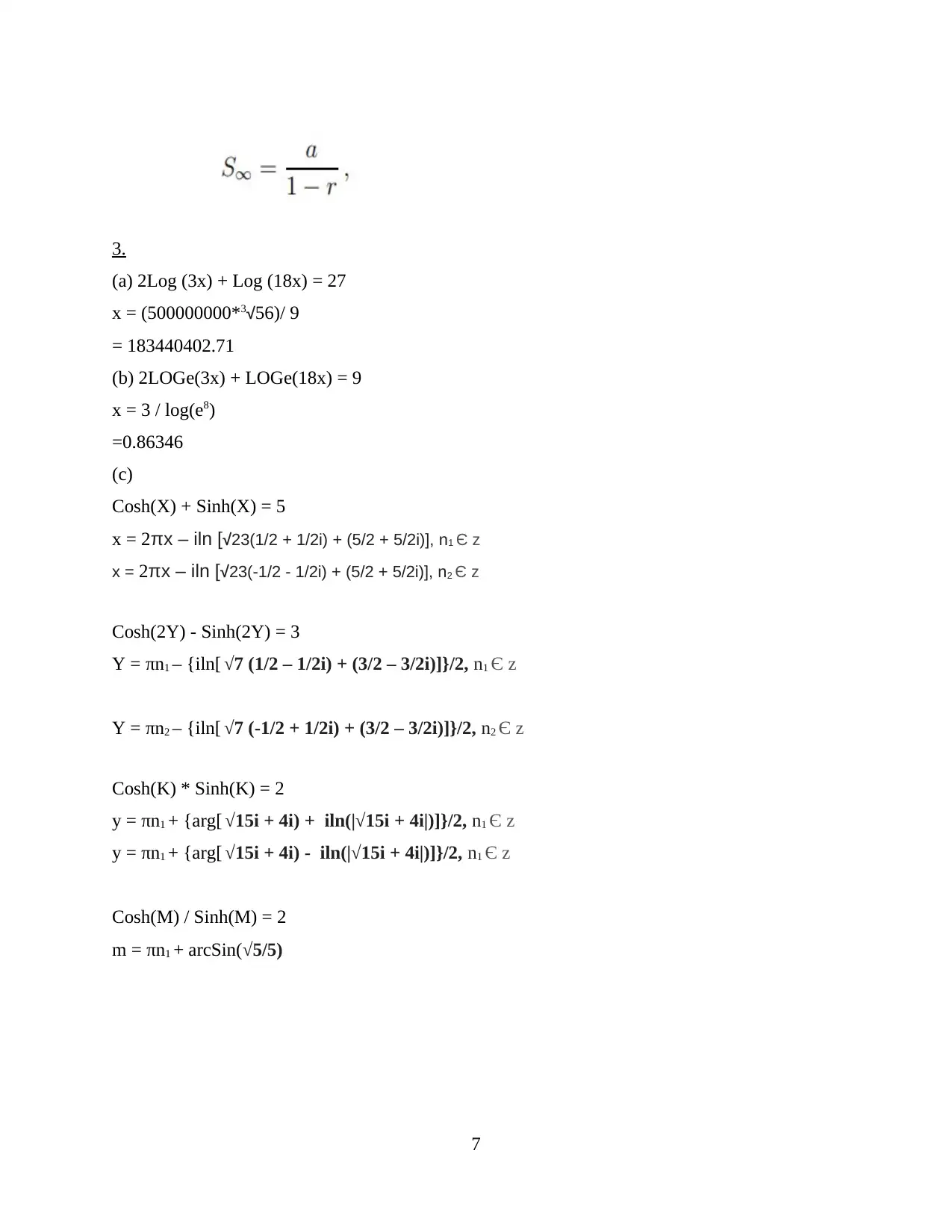
In each such case, should subtract small quantity out of 2, as well as take the successive total
quantity getting smaller than smaller. When one capable to add the infinitely terms, then
response ‘ought-to-be’ 2 or nearly 2.
6

3.
(a) 2Log (3x) + Log (18x) = 27
x = (500000000*3√56)/ 9
= 183440402.71
(b) 2LOGe(3x) + LOGe(18x) = 9
x = 3 / log(e8)
=0.86346
(c)
Cosh(X) + Sinh(X) = 5
x = 2πx – iln [√23(1/2 + 1/2i) + (5/2 + 5/2i)], n1 Є z
x = 2πx – iln [√23(-1/2 - 1/2i) + (5/2 + 5/2i)], n2 Є z
Cosh(2Y) - Sinh(2Y) = 3
Y = πn1 – {iln[ √7 (1/2 – 1/2i) + (3/2 – 3/2i)]}/2, n1 Є z
Y = πn2 – {iln[ √7 (-1/2 + 1/2i) + (3/2 – 3/2i)]}/2, n2 Є z
Cosh(K) * Sinh(K) = 2
y = πn1 + {arg[ √15i + 4i) + iln(|√15i + 4i|)]}/2, n1 Є z
y = πn1 + {arg[ √15i + 4i) - iln(|√15i + 4i|)]}/2, n1 Є z
Cosh(M) / Sinh(M) = 2
m = πn1 + arcSin(√5/5)
7

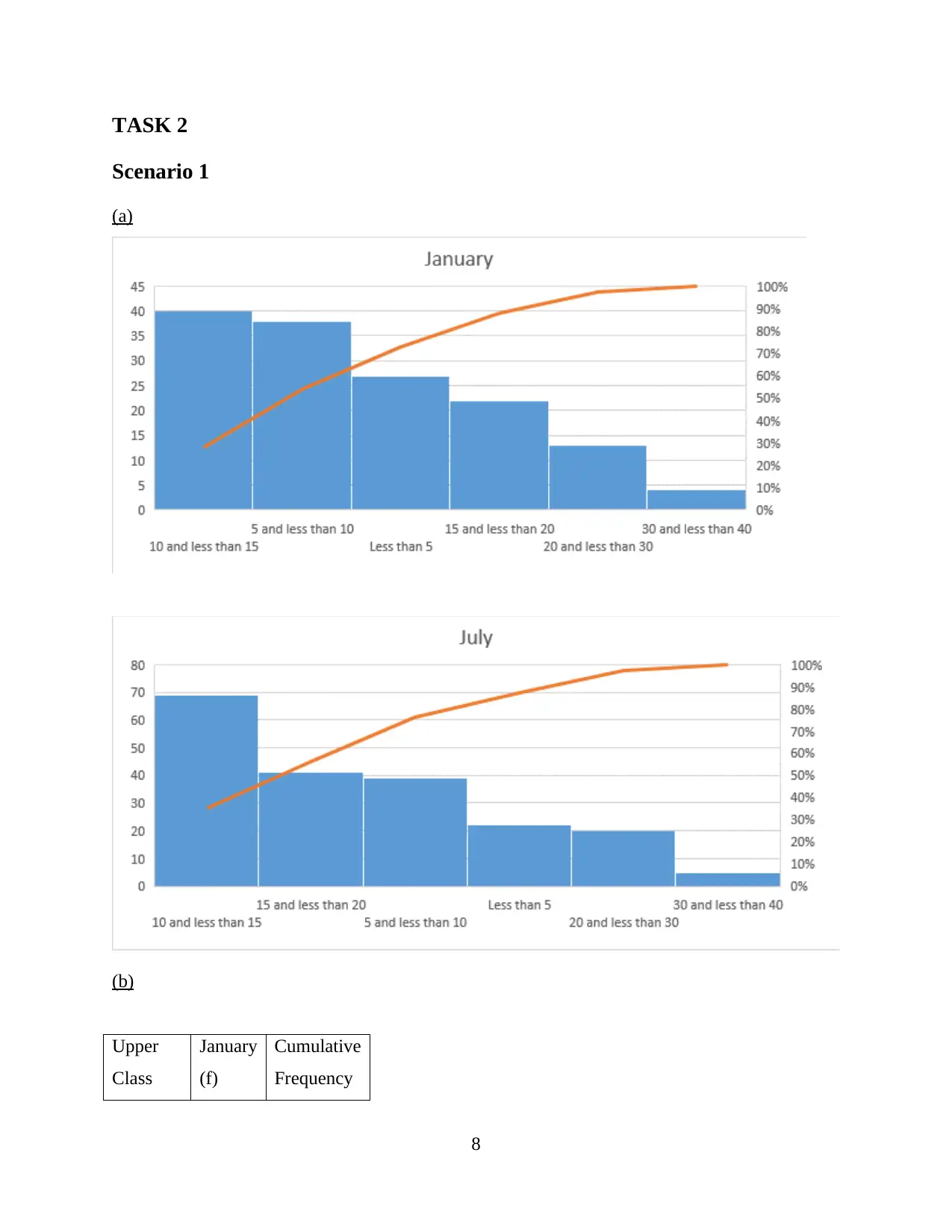
TASK 2
Scenario 1
(a)
(b)
Upper
Class
January
(f)
Cumulative
Frequency
8

boundary
4 27 27
9 38 65
14 40 105
19 22 127
29 13 140
39 4 144
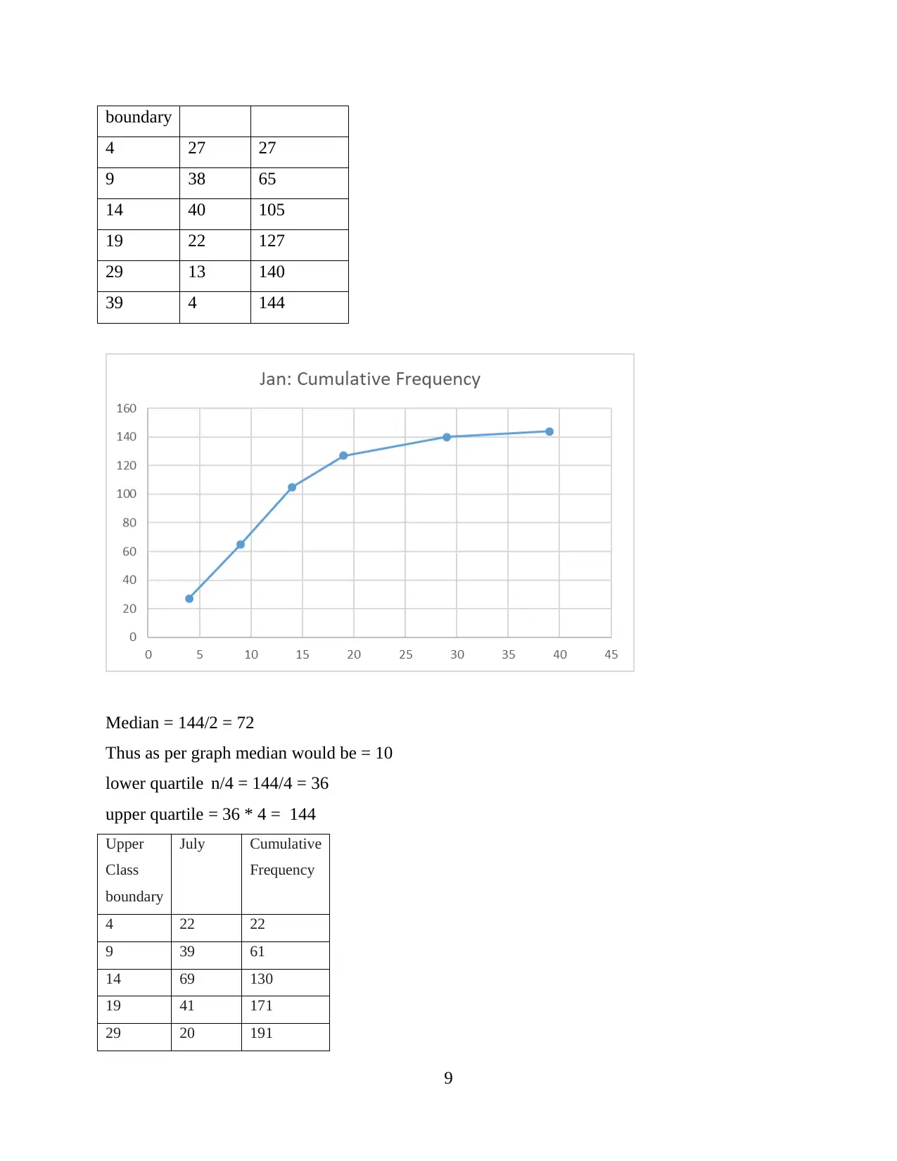
Median = 144/2 = 72
Thus as per graph median would be = 10
lower quartile n/4 = 144/4 = 36
upper quartile = 36 * 4 = 144
Upper
Class
boundary
July Cumulative
Frequency
4 22 22
9 39 61
14 69 130
19 41 171
29 20 191
9

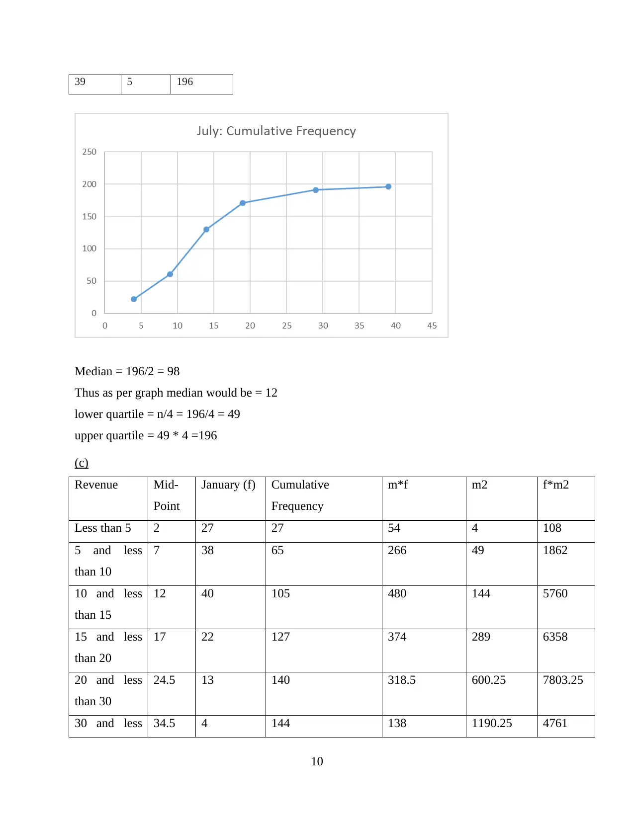
39 5 196
Median = 196/2 = 98
Thus as per graph median would be = 12
lower quartile = n/4 = 196/4 = 49
upper quartile = 49 * 4 =196
(c)
Revenue Mid-
Point
January (f) Cumulative
Frequency
m*f m2 f*m2
Less than 5 2 27 27 54 4 108
5 and less
than 10
7 38 65 266 49 1862
10 and less
than 15
12 40 105 480 144 5760
15 and less
than 20
17 22 127 374 289 6358
20 and less
than 30
24.5 13 140 318.5 600.25 7803.25
30 and less 34.5 4 144 138 1190.25 4761
10

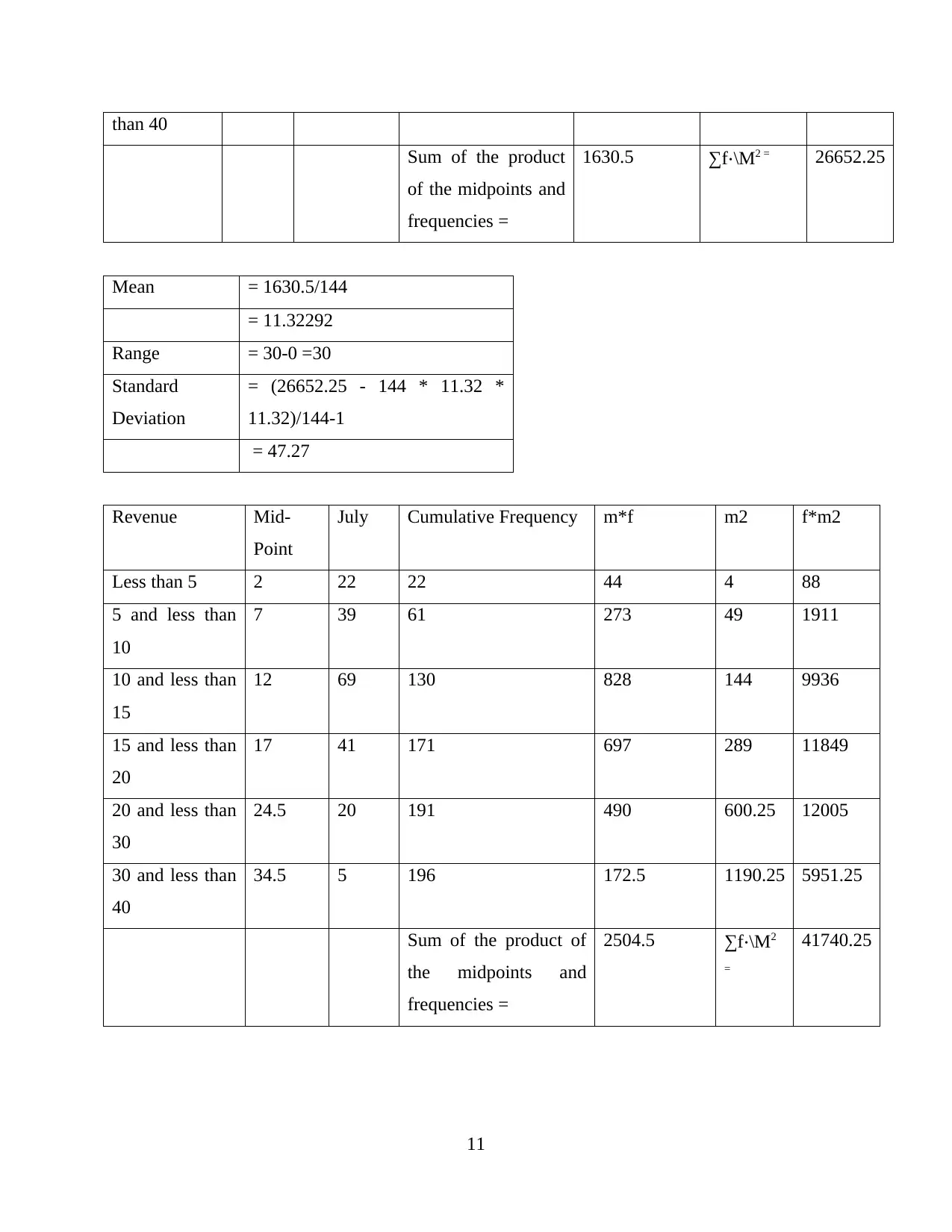
than 40
Sum of the product
of the midpoints and
frequencies =
1630.5 ∑f⋅\M2 = 26652.25
Mean = 1630.5/144
= 11.32292
Range = 30-0 =30
Standard
Deviation
= (26652.25 - 144 * 11.32 *
11.32)/144-1
= 47.27
Revenue Mid-
Point
July Cumulative Frequency m*f m2 f*m2
Less than 5 2 22 22 44 4 88
5 and less than
10
7 39 61 273 49 1911
10 and less than
15
12 69 130 828 144 9936
15 and less than
20
17 41 171 697 289 11849
20 and less than
30
24.5 20 191 490 600.25 12005
30 and less than
40
34.5 5 196 172.5 1190.25 5951.25
Sum of the product of
the midpoints and
frequencies =
2504.5 ∑f⋅\M2
=
41740.25
11

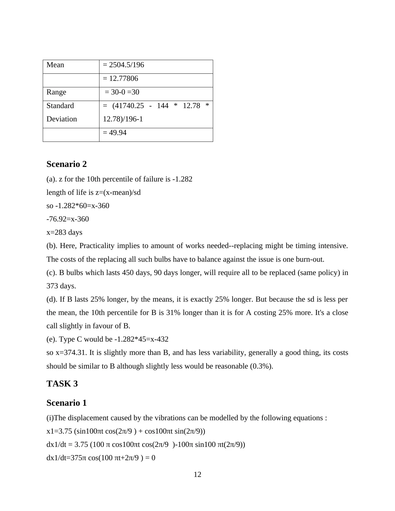
Mean = 2504.5/196
= 12.77806
Range = 30-0 =30
Standard
Deviation
= (41740.25 - 144 * 12.78 *
12.78)/196-1
= 49.94
Scenario 2
(a). z for the 10th percentile of failure is -1.282
length of life is z=(x-mean)/sd
so -1.282*60=x-360
-76.92=x-360
x=283 days
(b). Here, Practicality implies to amount of works needed--replacing might be timing intensive.
The costs of the replacing all such bulbs have to balance against the issue is one burn-out.
(c). B bulbs which lasts 450 days, 90 days longer, will require all to be replaced (same policy) in
373 days.
(d). If B lasts 25% longer, by the means, it is exactly 25% longer. But because the sd is less per
the mean, the 10th percentile for B is 31% longer than it is for A costing 25% more. It's a close
call slightly in favour of B.
(e). Type C would be -1.282*45=x-432
so x=374.31. It is slightly more than B, and has less variability, generally a good thing, its costs
should be similar to B although slightly less would be reasonable (0.3%).
TASK 3
Scenario 1
(i)The displacement caused by the vibrations can be modelled by the following equations :
x1=3.75 (sin100πt cos(2π/9 ) + cos100πt sin(2π/9))
dx1/dt = 3.75 (100 π cos100πt cos(2π/9 )-100π sin100 πt(2π/9))
dx1/dt=375π cos(100 πt+2π/9 ) = 0
12

cos(100 πt+2π/9 ) = 0
100πt+2π/9 = π/2
100πt = 5π/18
100 t = 5/18
t = 5/1800 seconds
(ii) x2=4.42 (sin100πt cos(2π/5 ) - cos100πt sin(2π/5))
dx2/dt = 4.42(100 π cos100πt cos(2π/5 )+100π sin100 πt(2π/5))
dx2/dt = 442π cos(100 πt-2π/5 ) = 0
442 cos(100 πt-2π/5 ) = 0
cos(100 πt-2π/5 ) = 0
100πt-2π/5 = π/2
100πt = 9π/10
100 t = 9/10
t = 9/1000 seconds
(iii)
-2=3.75 sin (100 πt+2π/9 )
sin (100 πt+2π/9 ) = -0.533333
100πt+2π/9 = arc sin(-0.533333)
t=1.8809/100π=0.00599 second
(iv)
-2=442 sin (100 πt-2π/5 )
sin (100 πt-2π/5 ) = -0.45249
100πt=0.78708
t=0.00251 seconds
R Sin(100πt+a)
x1=3.75 sin (100 πt+2π/9 )
x2=4.42 sin (100 πt-2π/5 )
13

x_1attains its max x_1 in 1/900 second after start.
x_2attains its max x_1 in 9/1000 second after start.
About 0.0095 second after start x_1 reaches -2mm
About 0.0025 second after start x_2 reaches -2mm
(v) A general wave equation is
x=A sin(2πRt+P)
x=Rsin (100πt+a)
Where R is the amplitude
t is the time
t x1 x2 x1+x2
0 2.411261 -4.20436 -1.7931
0.002 3.639093 -2.59892 1.040178
0.004 3.475833 9.81E-16 3.475833
0.006 1.98389 2.598915 4.582805
0.008 -0.26642 4.20436 3.937938
0.01 -2.41489 4.202632 1.787742
0.012 -3.64023 2.594392 -1.04584
0.014 -3.47405 -0.00559 -3.47964
0.016 -1.97986 -2.60343 -4.5833
0.018 0.271152 -4.20608 -3.93493
0.02 2.418516 -4.2009 -1.78238
14

Scenario 2
(i). From the figure,
Distance AB = √((40-0)^2+(0-(-40)^2+(-20-0)^2 )
= √((40)^2+ (40)^2+ (-20)^2 )
= √(1600+1600+400) = 60 meters (Distance AB)
(ii) The given section BC is to be drilled in the direction of vector 3i+4j+k
The vector equation of BC is :
(a-40) i + (b - 0) j + (0-(-20)) k
(a-40) i + b j + 20k
Compare this equation by c (3i+4j+k )
a - 40 = 3c
b = 4c
20 = c
a = 60 + 40 = 100
b = 80 , c = 20
The vector equation of AB is
40 i + 40 j - 20 k
The vector equation of BC is
60 i + 80 j + 20 k
We know that,
<AB , BC > = cosθAB BC
(iii). Denotes the norm of vector
cosθ=((40 i+40 j-20k)(60 i+80j+20k))/(√((40)^2+(40)^2+(20)^2 )
√((60)^2+(40)^2+(20)^2 ))
cosθ=(2400+3200-400)/(60 √10400)=52/61.14
cosθ=0.85050
θ=cos^(-1)( 0.85050)
θ=31.7339^0= 32^0
Angle between section AB and BC is 31.7339^0= 32^0
TASK 4
Scenario 1
(a.) Bending moment M = 3000 – 550 x – 20 x2
Solution
M = 3000 – 550 x – 20 x2
dm/dx = -550 – 40 x
15

equating dm/dx = 0 we have: -550 – 40 x = 0
so: 40x = - 550
x = -13.75
d2M /dx2 = -40
It is negative thus the given momentum function has local maxima at x = -13.75
The maximum value of function is given by:
M (x = -13.75) = 3000 – 550 x – 20 x2
M (x = -13.75) = 6781.25
The bending moment is zero at x = 4.664 .
(aii) The bending moment
(b.) Ө = 300 + 100 e^ (-0.1 t)
Ө is temperature in degree Celsius and t is time in minutes
Solution
At t = 0
Ө = 300 + 100 e^ (0) = 400
At t = 1
Ө = 300 + 100 e^ (-0.1*1) = 390
At t = 2
16

Ө = 300 + 100 e^ (-0.1*2) = 381
At t = 5
Ө = 300 + 100 e^ (-0.1*5) = 360
At t = ∞
Ө = 300 + 100 e^ (-0.1*∞) = 300
At t = -∞
Ө = 300 + 100 e^ (∞) = ∞
Thus value of temperature is positive for all values of t between -∞ and +∞
(C) log P + n log V – log C
Solution
P stands for pressure; V for volume and C is constant and n is known as index
log P + n log V = log C
By using the identity: a log x = log xa
log P + log Vn = log C
By identity: log a + log b = log ab we can write the above equation:
Log P Vn = log C
P Vn = C Hence proved
Also
log P =log C - n log V
Differentiating both sides with respect to P; we have:
1/P = -n (1/V) dV/d P
dV/d P = - (V/ n*P)
For n = 2 we have
dV/d P = - (V/ 2P)
17

Scenario 2
C = 16 t2 + 2t
Solution
(a. )
T 1 2 3 4 5 6 7 8
C 18 68 150 264 410 588 798 1040
(b)
The calculus can be used to provide the analytical solutions for the given condition. Using
concept of differentiation, it is possible to find the values of production time at which maximum
or minimum cost is obtained. The information helps in optimising the production cost by making
adjustments to the production time.
(C)
C = 16 t2 + 2t
Differentiating cost function with respect to time.
18

dC/dt = 32t + 2
Equating first derivative to zero
32t + 2 = 0
t = -0.062
Second derivative of cost function is:
d2c/dt2 = 32 Which is greater than zero.
It means at t = -0.06 minimum production cost is obtained which is £32.
(D).
The turning point is at t= -0.06 at which cost is minimum and beyond that time the cost function
becomes negative.
Scenario 3
Solution
Heat flow H = e3t
Where t is the temperature difference outside the building.
At t = -20 H = 8.75651E-27
At t = 0 H = 1
At t = 20 H = 1.14…. E26
19