Maths Coursework: Loan Calculations and Linear Programming Analysis
VerifiedAdded on 2023/06/10
|12
|3853
|371
Homework Assignment
AI Summary
This maths coursework solution addresses topics including loan payments, linear programming, and statistical analysis. It begins by calculating monthly loan payments under different interest rate scenarios and determines the affordability of loans. The coursework then delves into linear programming, optimizing production based on demand constraints and machine hour availability. Scenarios involving maximum demand and machine hour limitations are analyzed. Finally, the solution includes statistical analysis of exam grades, comparing the impact of study hours on performance in different subjects and discussing data inconsistencies. The analysis involves hypothesis testing and regression analysis to draw conclusions about the significance of study habits.
MATHS COURSEWORK – Sumair Saigal
Question 1
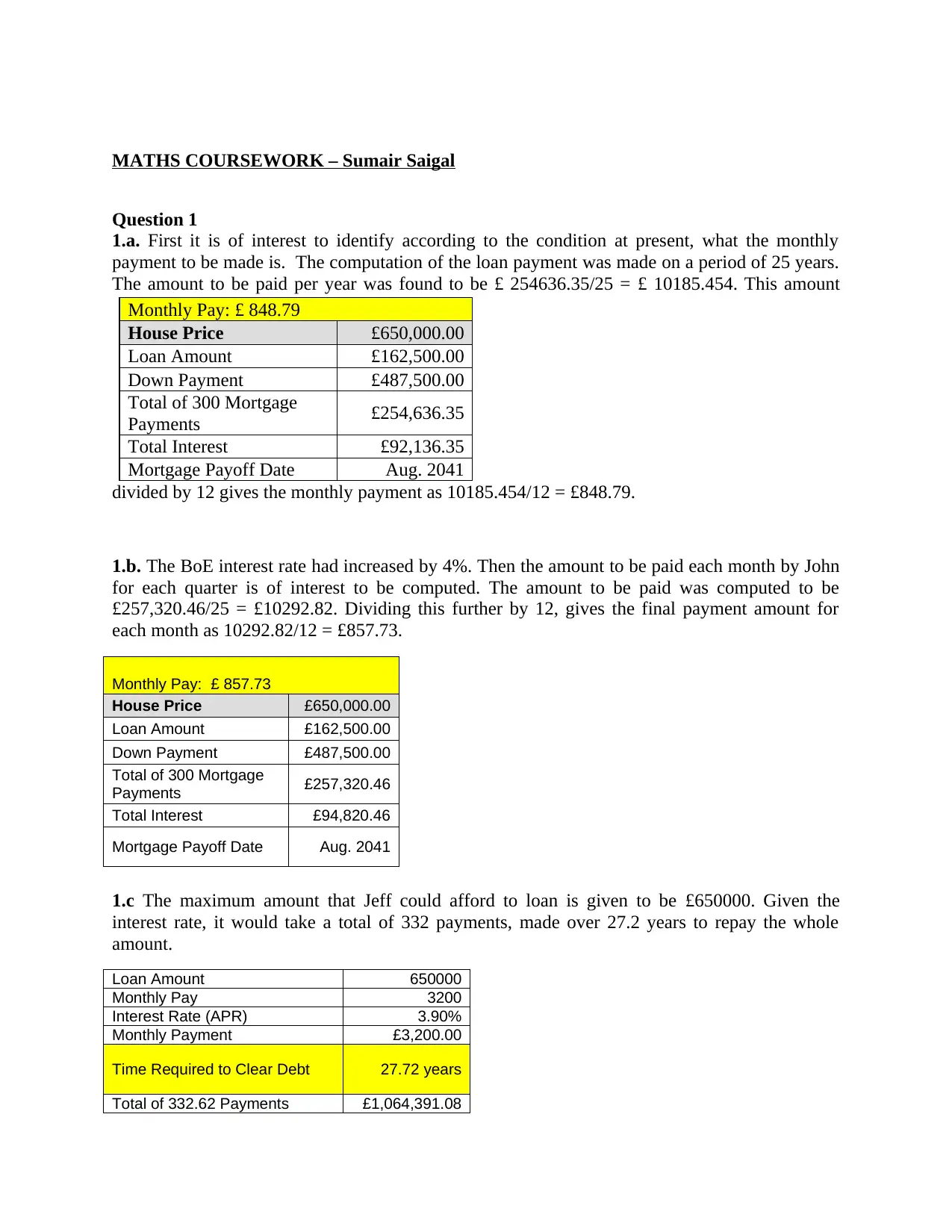
1.a. First it is of interest to identify according to the condition at present, what the monthly
payment to be made is. The computation of the loan payment was made on a period of 25 years.
The amount to be paid per year was found to be £ 254636.35/25 = £ 10185.454. This amount
divided by 12 gives the monthly payment as 10185.454/12 = £848.79.
1.b. The BoE interest rate had increased by 4%. Then the amount to be paid each month by John
for each quarter is of interest to be computed. The amount to be paid was computed to be
£257,320.46/25 = £10292.82. Dividing this further by 12, gives the final payment amount for
each month as 10292.82/12 = £857.73.
Monthly Pay: £ 857.73
House Price £650,000.00
Loan Amount £162,500.00
Down Payment £487,500.00
Total of 300 Mortgage
Payments £257,320.46
Total Interest £94,820.46
Mortgage Payoff Date Aug. 2041
1.c The maximum amount that Jeff could afford to loan is given to be £650000. Given the
interest rate, it would take a total of 332 payments, made over 27.2 years to repay the whole
amount.
Loan Amount 650000
Monthly Pay 3200
Interest Rate (APR) 3.90%
Monthly Payment £3,200.00
Time Required to Clear Debt 27.72 years
Total of 332.62 Payments £1,064,391.08
Monthly Pay: £ 848.79
House Price £650,000.00
Loan Amount £162,500.00
Down Payment £487,500.00
Total of 300 Mortgage
Payments £254,636.35
Total Interest £92,136.35
Mortgage Payoff Date Aug. 2041
Paraphrase This Document
Need a fresh take? Get an instant paraphrase of this document with our AI Paraphraser
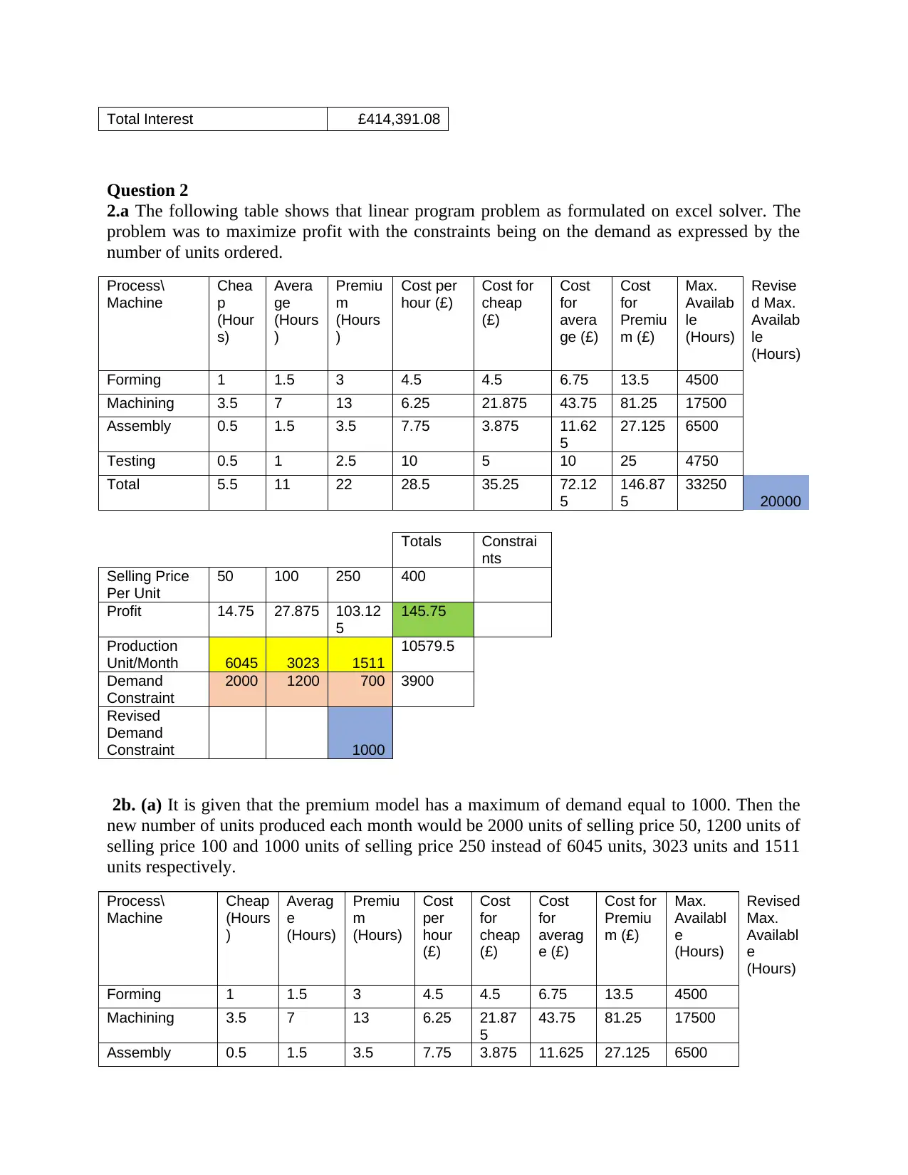
Total Interest £414,391.08
Question 2
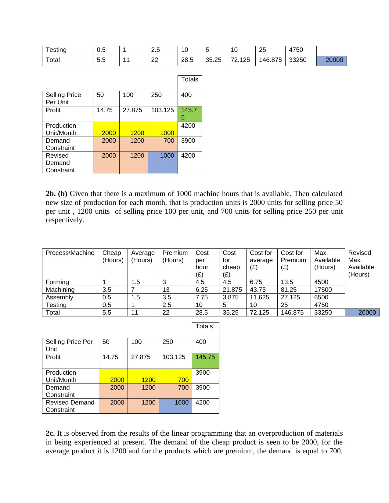
2.a The following table shows that linear program problem as formulated on excel solver. The
problem was to maximize profit with the constraints being on the demand as expressed by the
number of units ordered.
Process\
Machine
Chea
p
(Hour
s)
Avera
ge
(Hours
)
Premiu
m
(Hours
)
Cost per
hour (£)
Cost for
cheap
(£)
Cost
for
avera
ge (£)
Cost
for
Premiu
m (£)
Max.
Availab
le
(Hours)
Revise
d Max.
Availab
le
(Hours)
Forming 1 1.5 3 4.5 4.5 6.75 13.5 4500
Machining 3.5 7 13 6.25 21.875 43.75 81.25 17500
Assembly 0.5 1.5 3.5 7.75 3.875 11.62
5
27.125 6500
Testing 0.5 1 2.5 10 5 10 25 4750
Total 5.5 11 22 28.5 35.25 72.12
5
146.87
5
33250
20000
Totals Constrai
nts
Selling Price
Per Unit
50 100 250 400
Profit 14.75 27.875 103.12
5
145.75
Production
Unit/Month 6045 3023 1511
10579.5
Demand
Constraint
2000 1200 700 3900
Revised
Demand
Constraint 1000
2b. (a) It is given that the premium model has a maximum of demand equal to 1000. Then the
new number of units produced each month would be 2000 units of selling price 50, 1200 units of
selling price 100 and 1000 units of selling price 250 instead of 6045 units, 3023 units and 1511
units respectively.
Process\
Machine
Cheap
(Hours
)
Averag
e
(Hours)
Premiu
m
(Hours)
Cost
per
hour
(£)
Cost
for
cheap
(£)
Cost
for
averag
e (£)
Cost for
Premiu
m (£)
Max.
Availabl
e
(Hours)
Revised
Max.
Availabl
e
(Hours)
Forming 1 1.5 3 4.5 4.5 6.75 13.5 4500
Machining 3.5 7 13 6.25 21.87
5
43.75 81.25 17500
Assembly 0.5 1.5 3.5 7.75 3.875 11.625 27.125 6500
Testing 0.5 1 2.5 10 5 10 25 4750
Total 5.5 11 22 28.5 35.25 72.125 146.875 33250 20000
Totals
Selling Price
Per Unit
50 100 250 400
Profit 14.75 27.875 103.125 145.7
5
Production
Unit/Month 2000 1200 1000
4200
Demand
Constraint
2000 1200 700 3900
Revised
Demand
Constraint
2000 1200 1000 4200
2b. (b) Given that there is a maximum of 1000 machine hours that is available. Then calculated
new size of production for each month, that is production units is 2000 units for selling price 50
per unit , 1200 units of selling price 100 per unit, and 700 units for selling price 250 per unit
respectively.
Process\Machine Cheap
(Hours)
Average
(Hours)
Premium
(Hours)
Cost
per
hour
(£)
Cost
for
cheap
(£)
Cost for
average
(£)
Cost for
Premium
(£)
Max.
Available
(Hours)
Revised
Max.
Available
(Hours)
Forming 1 1.5 3 4.5 4.5 6.75 13.5 4500
Machining 3.5 7 13 6.25 21.875 43.75 81.25 17500
Assembly 0.5 1.5 3.5 7.75 3.875 11.625 27.125 6500
Testing 0.5 1 2.5 10 5 10 25 4750
Total 5.5 11 22 28.5 35.25 72.125 146.875 33250 20000
Totals
Selling Price Per
Unit
50 100 250 400
Profit 14.75 27.875 103.125 145.75
Production
Unit/Month 2000 1200 700
3900
Demand
Constraint
2000 1200 700 3900
Revised Demand
Constraint
2000 1200 1000 4200
2c. It is observed from the results of the linear programming that an overproduction of materials
in being experienced at present. The demand of the cheap product is seen to be 2000, for the
average product it is 1200 and for the products which are premium, the demand is equal to 700.
Total 5.5 11 22 28.5 35.25 72.125 146.875 33250 20000
Totals
Selling Price
Per Unit
50 100 250 400
Profit 14.75 27.875 103.125 145.7
5
Production
Unit/Month 2000 1200 1000
4200
Demand
Constraint
2000 1200 700 3900
Revised
Demand
Constraint
2000 1200 1000 4200
2b. (b) Given that there is a maximum of 1000 machine hours that is available. Then calculated
new size of production for each month, that is production units is 2000 units for selling price 50
per unit , 1200 units of selling price 100 per unit, and 700 units for selling price 250 per unit
respectively.
Process\Machine Cheap
(Hours)
Average
(Hours)
Premium
(Hours)
Cost
per
hour
(£)
Cost
for
cheap
(£)
Cost for
average
(£)
Cost for
Premium
(£)
Max.
Available
(Hours)
Revised
Max.
Available
(Hours)
Forming 1 1.5 3 4.5 4.5 6.75 13.5 4500
Machining 3.5 7 13 6.25 21.875 43.75 81.25 17500
Assembly 0.5 1.5 3.5 7.75 3.875 11.625 27.125 6500
Testing 0.5 1 2.5 10 5 10 25 4750
Total 5.5 11 22 28.5 35.25 72.125 146.875 33250 20000
Totals
Selling Price Per
Unit
50 100 250 400
Profit 14.75 27.875 103.125 145.75
Production
Unit/Month 2000 1200 700
3900
Demand
Constraint
2000 1200 700 3900
Revised Demand
Constraint
2000 1200 1000 4200
2c. It is observed from the results of the linear programming that an overproduction of materials
in being experienced at present. The demand of the cheap product is seen to be 2000, for the
average product it is 1200 and for the products which are premium, the demand is equal to 700.
⊘ This is a preview!⊘
Do you want full access?
Subscribe today to unlock all pages.

Trusted by 1+ million students worldwide
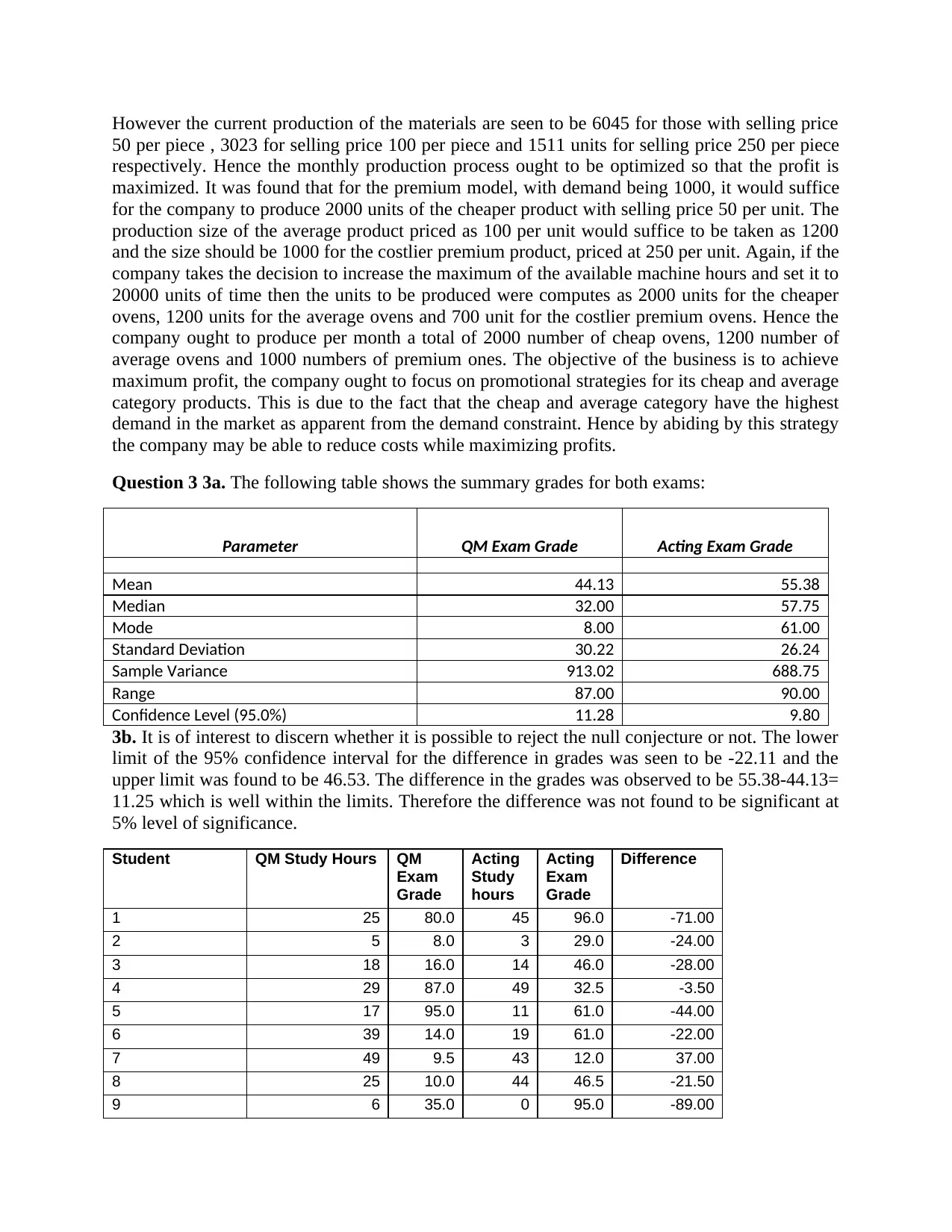
However the current production of the materials are seen to be 6045 for those with selling price
50 per piece , 3023 for selling price 100 per piece and 1511 units for selling price 250 per piece
respectively. Hence the monthly production process ought to be optimized so that the profit is
maximized. It was found that for the premium model, with demand being 1000, it would suffice
for the company to produce 2000 units of the cheaper product with selling price 50 per unit. The
production size of the average product priced as 100 per unit would suffice to be taken as 1200
and the size should be 1000 for the costlier premium product, priced at 250 per unit. Again, if the
company takes the decision to increase the maximum of the available machine hours and set it to
20000 units of time then the units to be produced were computes as 2000 units for the cheaper
ovens, 1200 units for the average ovens and 700 unit for the costlier premium ovens. Hence the
company ought to produce per month a total of 2000 number of cheap ovens, 1200 number of
average ovens and 1000 numbers of premium ones. The objective of the business is to achieve
maximum profit, the company ought to focus on promotional strategies for its cheap and average
category products. This is due to the fact that the cheap and average category have the highest
demand in the market as apparent from the demand constraint. Hence by abiding by this strategy
the company may be able to reduce costs while maximizing profits.
Question 3 3a. The following table shows the summary grades for both exams:
Parameter QM Exam Grade Acting Exam Grade
Mean 44.13 55.38
Median 32.00 57.75
Mode 8.00 61.00
Standard Deviation 30.22 26.24
Sample Variance 913.02 688.75
Range 87.00 90.00
Confidence Level (95.0%) 11.28 9.80
3b. It is of interest to discern whether it is possible to reject the null conjecture or not. The lower
limit of the 95% confidence interval for the difference in grades was seen to be -22.11 and the
upper limit was found to be 46.53. The difference in the grades was observed to be 55.38-44.13=
11.25 which is well within the limits. Therefore the difference was not found to be significant at
5% level of significance.
Student QM Study Hours QM
Exam
Grade
Acting
Study
hours
Acting
Exam
Grade
Difference
1 25 80.0 45 96.0 -71.00
2 5 8.0 3 29.0 -24.00
3 18 16.0 14 46.0 -28.00
4 29 87.0 49 32.5 -3.50
5 17 95.0 11 61.0 -44.00
6 39 14.0 19 61.0 -22.00
7 49 9.5 43 12.0 37.00
8 25 10.0 44 46.5 -21.50
9 6 35.0 0 95.0 -89.00
Paraphrase This Document
Need a fresh take? Get an instant paraphrase of this document with our AI Paraphraser
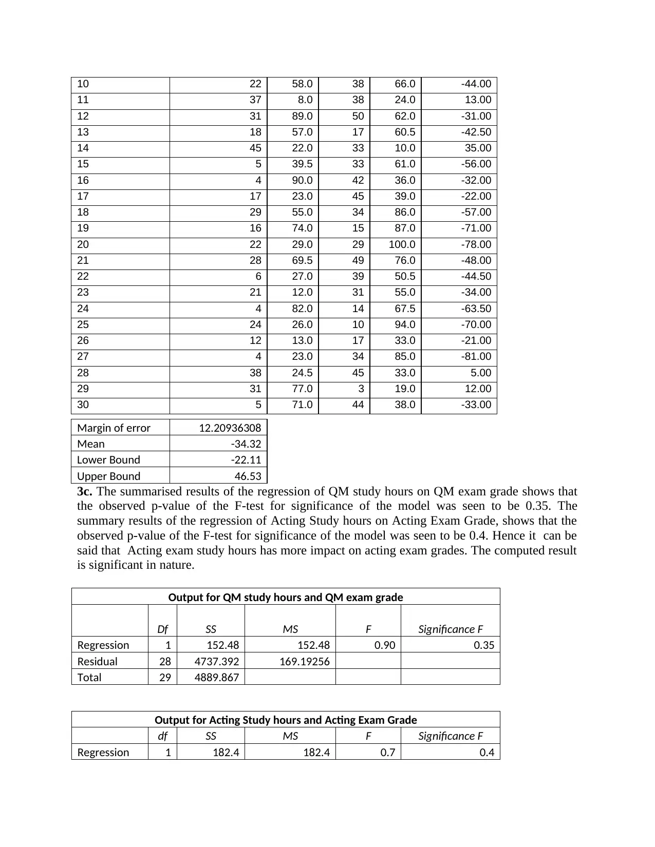
10 22 58.0 38 66.0 -44.00
11 37 8.0 38 24.0 13.00
12 31 89.0 50 62.0 -31.00
13 18 57.0 17 60.5 -42.50
14 45 22.0 33 10.0 35.00
15 5 39.5 33 61.0 -56.00
16 4 90.0 42 36.0 -32.00
17 17 23.0 45 39.0 -22.00
18 29 55.0 34 86.0 -57.00
19 16 74.0 15 87.0 -71.00
20 22 29.0 29 100.0 -78.00
21 28 69.5 49 76.0 -48.00
22 6 27.0 39 50.5 -44.50
23 21 12.0 31 55.0 -34.00
24 4 82.0 14 67.5 -63.50
25 24 26.0 10 94.0 -70.00
26 12 13.0 17 33.0 -21.00
27 4 23.0 34 85.0 -81.00
28 38 24.5 45 33.0 5.00
29 31 77.0 3 19.0 12.00
30 5 71.0 44 38.0 -33.00
Margin of error 12.20936308
Mean -34.32
Lower Bound -22.11
Upper Bound 46.53
3c. The summarised results of the regression of QM study hours on QM exam grade shows that
the observed p-value of the F-test for significance of the model was seen to be 0.35. The
summary results of the regression of Acting Study hours on Acting Exam Grade, shows that the
observed p-value of the F-test for significance of the model was seen to be 0.4. Hence it can be
said that Acting exam study hours has more impact on acting exam grades. The computed result
is significant in nature.
Output for QM study hours and QM exam grade
Df SS MS F Significance F
Regression 1 152.48 152.48 0.90 0.35
Residual 28 4737.392 169.19256
Total 29 4889.867
Output for Acting Study hours and Acting Exam Grade
df SS MS F Significance F
Regression 1 182.4 182.4 0.7 0.4
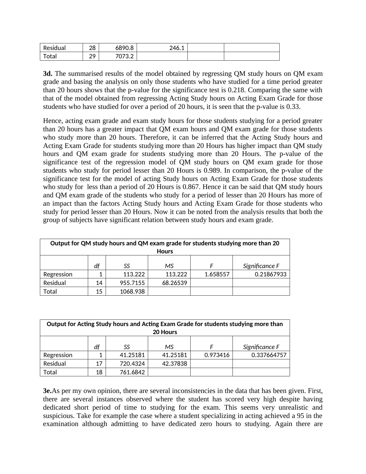
Residual 28 6890.8 246.1
Total 29 7073.2
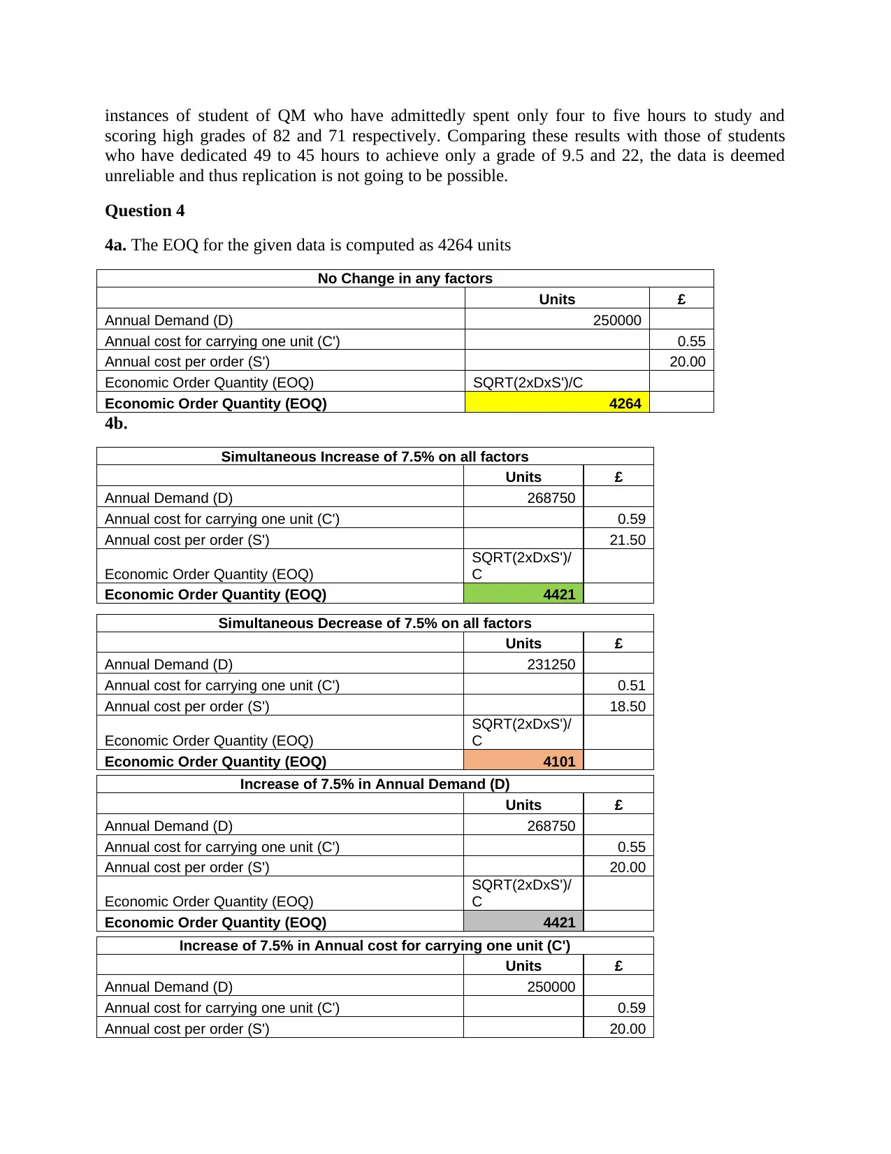
3d. The summarised results of the model obtained by regressing QM study hours on QM exam
grade and basing the analysis on only those students who have studied for a time period greater
than 20 hours shows that the p-value for the significance test is 0.218. Comparing the same with
that of the model obtained from regressing Acting Study hours on Acting Exam Grade for those
students who have studied for over a period of 20 hours, it is seen that the p-value is 0.33.
Hence, acting exam grade and exam study hours for those students studying for a period greater
than 20 hours has a greater impact that QM exam hours and QM exam grade for those students
who study more than 20 hours. Therefore, it can be inferred that the Acting Study hours and
Acting Exam Grade for students studying more than 20 Hours has higher impact than QM study
hours and QM exam grade for students studying more than 20 Hours. The p-value of the
significance test of the regression model of QM study hours on QM exam grade for those
students who study for period lesser than 20 Hours is 0.989. In comparison, the p-value of the
significance test for the model of acting Study hours on Acting Exam Grade for those students
who study for less than a period of 20 Hours is 0.867. Hence it can be said that QM study hours
and QM exam grade of the students who study for a period of lesser than 20 Hours has more of
an impact than the factors Acting Study hours and Acting Exam Grade for those students who
study for period lesser than 20 Hours. Now it can be noted from the analysis results that both the
group of subjects have significant relation between study hours and exam grade.
3e.As per my own opinion, there are several inconsistencies in the data that has been given. First,
there are several instances observed where the student has scored very high despite having
dedicated short period of time to studying for the exam. This seems very unrealistic and
suspicious. Take for example the case where a student specializing in acting achieved a 95 in the
examination although admitting to have dedicated zero hours to studying. Again there are
Output for QM study hours and QM exam grade for students studying more than 20
Hours
df SS MS F Significance F
Regression 1 113.222 113.222 1.658557 0.21867933
Residual 14 955.7155 68.26539
Total 15 1068.938
Output for Acting Study hours and Acting Exam Grade for students studying more than
20 Hours
df SS MS F Significance F
Regression 1 41.25181 41.25181 0.973416 0.337664757
Residual 17 720.4324 42.37838
Total 18 761.6842
⊘ This is a preview!⊘
Do you want full access?
Subscribe today to unlock all pages.

Trusted by 1+ million students worldwide
instances of student of QM who have admittedly spent only four to five hours to study and
scoring high grades of 82 and 71 respectively. Comparing these results with those of students
who have dedicated 49 to 45 hours to achieve only a grade of 9.5 and 22, the data is deemed
unreliable and thus replication is not going to be possible.
Question 4
4a. The EOQ for the given data is computed as 4264 units
No Change in any factors
Units £
Annual Demand (D) 250000
Annual cost for carrying one unit (C') 0.55
Annual cost per order (S') 20.00
Economic Order Quantity (EOQ) SQRT(2xDxS')/C
Economic Order Quantity (EOQ) 4264
4b.
Simultaneous Increase of 7.5% on all factors
Units £
Annual Demand (D) 268750
Annual cost for carrying one unit (C') 0.59
Annual cost per order (S') 21.50
Economic Order Quantity (EOQ)
SQRT(2xDxS')/
C
Economic Order Quantity (EOQ) 4421
Simultaneous Decrease of 7.5% on all factors
Units £
Annual Demand (D) 231250
Annual cost for carrying one unit (C') 0.51
Annual cost per order (S') 18.50
Economic Order Quantity (EOQ)
SQRT(2xDxS')/
C
Economic Order Quantity (EOQ) 4101
Increase of 7.5% in Annual Demand (D)
Units £
Annual Demand (D) 268750
Annual cost for carrying one unit (C') 0.55
Annual cost per order (S') 20.00
Economic Order Quantity (EOQ)
SQRT(2xDxS')/
C
Economic Order Quantity (EOQ) 4421
Increase of 7.5% in Annual cost for carrying one unit (C')
Units £
Annual Demand (D) 250000
Annual cost for carrying one unit (C') 0.59
Annual cost per order (S') 20.00
Paraphrase This Document
Need a fresh take? Get an instant paraphrase of this document with our AI Paraphraser
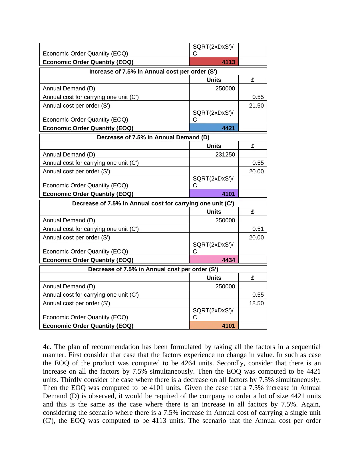
Economic Order Quantity (EOQ)
SQRT(2xDxS')/
C
Economic Order Quantity (EOQ) 4113
Increase of 7.5% in Annual cost per order (S')
Units £
Annual Demand (D) 250000
Annual cost for carrying one unit (C') 0.55
Annual cost per order (S') 21.50
Economic Order Quantity (EOQ)
SQRT(2xDxS')/
C
Economic Order Quantity (EOQ) 4421
Decrease of 7.5% in Annual Demand (D)
Units £
Annual Demand (D) 231250
Annual cost for carrying one unit (C') 0.55
Annual cost per order (S') 20.00
Economic Order Quantity (EOQ)
SQRT(2xDxS')/
C
Economic Order Quantity (EOQ) 4101
Decrease of 7.5% in Annual cost for carrying one unit (C')
Units £
Annual Demand (D) 250000
Annual cost for carrying one unit (C') 0.51
Annual cost per order (S') 20.00
Economic Order Quantity (EOQ)
SQRT(2xDxS')/
C
Economic Order Quantity (EOQ) 4434
Decrease of 7.5% in Annual cost per order (S')
Units £
Annual Demand (D) 250000
Annual cost for carrying one unit (C') 0.55
Annual cost per order (S') 18.50
Economic Order Quantity (EOQ)
SQRT(2xDxS')/
C
Economic Order Quantity (EOQ) 4101
4c. The plan of recommendation has been formulated by taking all the factors in a sequential
manner. First consider that case that the factors experience no change in value. In such as case
the EOQ of the product was computed to be 4264 units. Secondly, consider that there is an
increase on all the factors by 7.5% simultaneously. Then the EOQ was computed to be 4421
units. Thirdly consider the case where there is a decrease on all factors by 7.5% simultaneously.
Then the EOQ was computed to be 4101 units. Given the case that a 7.5% increase in Annual
Demand (D) is observed, it would be required of the company to order a lot of size 4421 units
and this is the same as the case where there is an increase in all factors by 7.5%. Again,
considering the scenario where there is a 7.5% increase in Annual cost of carrying a single unit
(C'), the EOQ was computed to be 4113 units. The scenario that the Annual cost per order
SQRT(2xDxS')/
C
Economic Order Quantity (EOQ) 4113
Increase of 7.5% in Annual cost per order (S')
Units £
Annual Demand (D) 250000
Annual cost for carrying one unit (C') 0.55
Annual cost per order (S') 21.50
Economic Order Quantity (EOQ)
SQRT(2xDxS')/
C
Economic Order Quantity (EOQ) 4421
Decrease of 7.5% in Annual Demand (D)
Units £
Annual Demand (D) 231250
Annual cost for carrying one unit (C') 0.55
Annual cost per order (S') 20.00
Economic Order Quantity (EOQ)
SQRT(2xDxS')/
C
Economic Order Quantity (EOQ) 4101
Decrease of 7.5% in Annual cost for carrying one unit (C')
Units £
Annual Demand (D) 250000
Annual cost for carrying one unit (C') 0.51
Annual cost per order (S') 20.00
Economic Order Quantity (EOQ)
SQRT(2xDxS')/
C
Economic Order Quantity (EOQ) 4434
Decrease of 7.5% in Annual cost per order (S')
Units £
Annual Demand (D) 250000
Annual cost for carrying one unit (C') 0.55
Annual cost per order (S') 18.50
Economic Order Quantity (EOQ)
SQRT(2xDxS')/
C
Economic Order Quantity (EOQ) 4101
4c. The plan of recommendation has been formulated by taking all the factors in a sequential
manner. First consider that case that the factors experience no change in value. In such as case
the EOQ of the product was computed to be 4264 units. Secondly, consider that there is an
increase on all the factors by 7.5% simultaneously. Then the EOQ was computed to be 4421
units. Thirdly consider the case where there is a decrease on all factors by 7.5% simultaneously.
Then the EOQ was computed to be 4101 units. Given the case that a 7.5% increase in Annual
Demand (D) is observed, it would be required of the company to order a lot of size 4421 units
and this is the same as the case where there is an increase in all factors by 7.5%. Again,
considering the scenario where there is a 7.5% increase in Annual cost of carrying a single unit
(C'), the EOQ was computed to be 4113 units. The scenario that the Annual cost per order
increases by 7.5% requires the company to counter with an EOQ equal to 4421 units and a
decrease of 7.5% on the other hand calls for the EOQ to be set as 4101 units. This is similar to
the cases when there was simultaneous change in all the factors by 7.5% simultaneously. The
decrease in the Annual price for carrying a single unit (C’) by 7.5% means that the EOQ should
be 4434 units. Finally, a decrease in Annual cost per order (S') by 7.5% means that EOQ should
be 4010 units. Now it can be seen through the course of the entire analysis of the numbers that
Annual Demand (D) has the most impact on EOQ and the changes it experiences. Another aspect
which is also affected by Annual Demand is the Annual cost per order (S’).
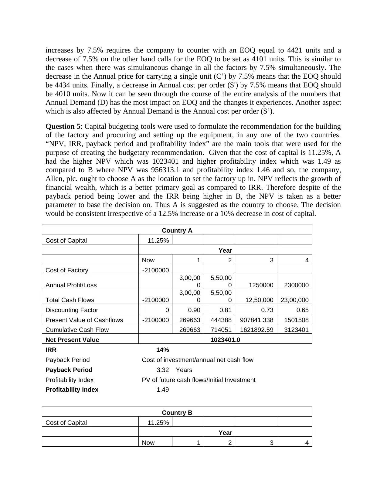
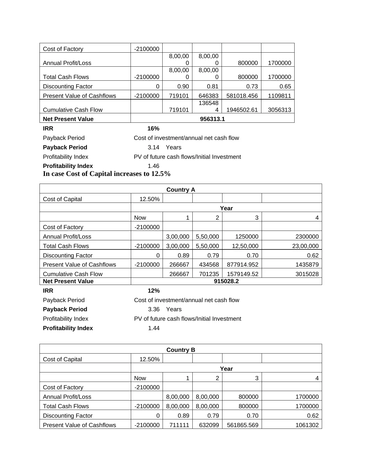
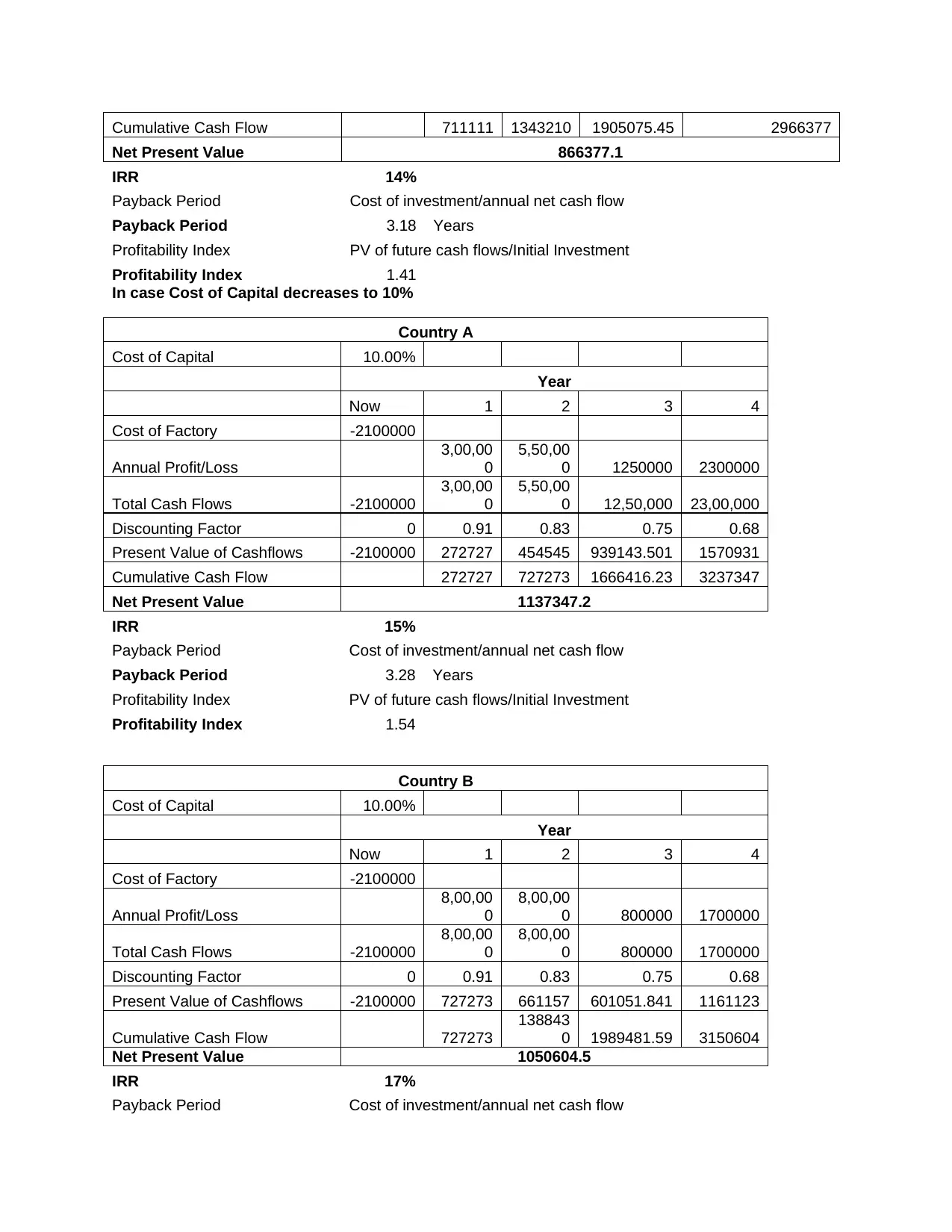
Question 5: Capital budgeting tools were used to formulate the recommendation for the building
of the factory and procuring and setting up the equipment, in any one of the two countries.
“NPV, IRR, payback period and profitability index” are the main tools that were used for the
purpose of creating the budgetary recommendation. Given that the cost of capital is 11.25%, A
had the higher NPV which was 1023401 and higher profitability index which was 1.49 as
compared to B where NPV was 956313.1 and profitability index 1.46 and so, the company,
Allen, plc. ought to choose A as the location to set the factory up in. NPV reflects the growth of
financial wealth, which is a better primary goal as compared to IRR. Therefore despite of the
payback period being lower and the IRR being higher in B, the NPV is taken as a better
parameter to base the decision on. Thus A is suggested as the country to choose. The decision
would be consistent irrespective of a 12.5% increase or a 10% decrease in cost of capital.
Country A
Cost of Capital 11.25%
Year
Now 1 2 3 4
Cost of Factory -2100000
Annual Profit/Loss
3,00,00
0
5,50,00
0 1250000 2300000
Total Cash Flows -2100000
3,00,00
0
5,50,00
0 12,50,000 23,00,000
Discounting Factor 0 0.90 0.81 0.73 0.65
Present Value of Cashflows -2100000 269663 444388 907841.338 1501508
Cumulative Cash Flow 269663 714051 1621892.59 3123401
Net Present Value 1023401.0
IRR 14%
Payback Period Cost of investment/annual net cash flow
Payback Period 3.32 Years
Profitability Index PV of future cash flows/Initial Investment
Profitability Index 1.49
Country B
Cost of Capital 11.25%
Year
Now 1 2 3 4
⊘ This is a preview!⊘
Do you want full access?
Subscribe today to unlock all pages.

Trusted by 1+ million students worldwide
Cost of Factory -2100000
Annual Profit/Loss
8,00,00
0
8,00,00
0 800000 1700000
Total Cash Flows -2100000
8,00,00
0
8,00,00
0 800000 1700000
Discounting Factor 0 0.90 0.81 0.73 0.65
Present Value of Cashflows -2100000 719101 646383 581018.456 1109811
Cumulative Cash Flow 719101
136548
4 1946502.61 3056313
Net Present Value 956313.1
IRR 16%
Payback Period Cost of investment/annual net cash flow
Payback Period 3.14 Years
Profitability Index PV of future cash flows/Initial Investment
Profitability Index 1.46
In case Cost of Capital increases to 12.5%
Country A
Cost of Capital 12.50%
Year
Now 1 2 3 4
Cost of Factory -2100000
Annual Profit/Loss 3,00,000 5,50,000 1250000 2300000
Total Cash Flows -2100000 3,00,000 5,50,000 12,50,000 23,00,000
Discounting Factor 0 0.89 0.79 0.70 0.62
Present Value of Cashflows -2100000 266667 434568 877914.952 1435879
Cumulative Cash Flow 266667 701235 1579149.52 3015028
Net Present Value 915028.2
IRR 12%
Payback Period Cost of investment/annual net cash flow
Payback Period 3.36 Years
Profitability Index PV of future cash flows/Initial Investment
Profitability Index 1.44
Country B
Cost of Capital 12.50%
Year
Now 1 2 3 4
Cost of Factory -2100000
Annual Profit/Loss 8,00,000 8,00,000 800000 1700000
Total Cash Flows -2100000 8,00,000 8,00,000 800000 1700000
Discounting Factor 0 0.89 0.79 0.70 0.62
Present Value of Cashflows -2100000 711111 632099 561865.569 1061302
Paraphrase This Document
Need a fresh take? Get an instant paraphrase of this document with our AI Paraphraser
Cumulative Cash Flow 711111 1343210 1905075.45 2966377
Net Present Value 866377.1
IRR 14%
Payback Period Cost of investment/annual net cash flow
Payback Period 3.18 Years
Profitability Index PV of future cash flows/Initial Investment
Profitability Index 1.41
In case Cost of Capital decreases to 10%
Country A
Cost of Capital 10.00%
Year
Now 1 2 3 4
Cost of Factory -2100000
Annual Profit/Loss
3,00,00
0
5,50,00
0 1250000 2300000
Total Cash Flows -2100000
3,00,00
0
5,50,00
0 12,50,000 23,00,000
Discounting Factor 0 0.91 0.83 0.75 0.68
Present Value of Cashflows -2100000 272727 454545 939143.501 1570931
Cumulative Cash Flow 272727 727273 1666416.23 3237347
Net Present Value 1137347.2
IRR 15%
Payback Period Cost of investment/annual net cash flow
Payback Period 3.28 Years
Profitability Index PV of future cash flows/Initial Investment
Profitability Index 1.54
Country B
Cost of Capital 10.00%
Year
Now 1 2 3 4
Cost of Factory -2100000
Annual Profit/Loss
8,00,00
0
8,00,00
0 800000 1700000
Total Cash Flows -2100000
8,00,00
0
8,00,00
0 800000 1700000
Discounting Factor 0 0.91 0.83 0.75 0.68
Present Value of Cashflows -2100000 727273 661157 601051.841 1161123
Cumulative Cash Flow 727273
138843
0 1989481.59 3150604
Net Present Value 1050604.5
IRR 17%
Payback Period Cost of investment/annual net cash flow

Payback Period 3.10 Years
Profitability Index PV of future cash flows/Initial Investment
Profitability Index 1.50
Profitability Index PV of future cash flows/Initial Investment
Profitability Index 1.50
⊘ This is a preview!⊘
Do you want full access?
Subscribe today to unlock all pages.

Trusted by 1+ million students worldwide
1 out of 12
Your All-in-One AI-Powered Toolkit for Academic Success.
+13062052269
info@desklib.com
Available 24*7 on WhatsApp / Email
![[object Object]](/_next/static/media/star-bottom.7253800d.svg)
Unlock your academic potential
Copyright © 2020–2025 A2Z Services. All Rights Reserved. Developed and managed by ZUCOL.


