MATLAB functions for distance conversion, time conversion, and quadratic equation roots

This article discusses three MATLAB functions for distance conversion, time conversion, and quadratic equation roots. It provides sample codes and outputs for each function. The distance conversion function converts miles and yards to kilometers. The time conversion function converts minutes to hours and minutes. The quadratic equation roots function finds the roots of a quadratic equation. The article also includes a discussion on the Taylor series of sin(x) and tan(x) and provides sample codes and outputs for each.

Sample question:
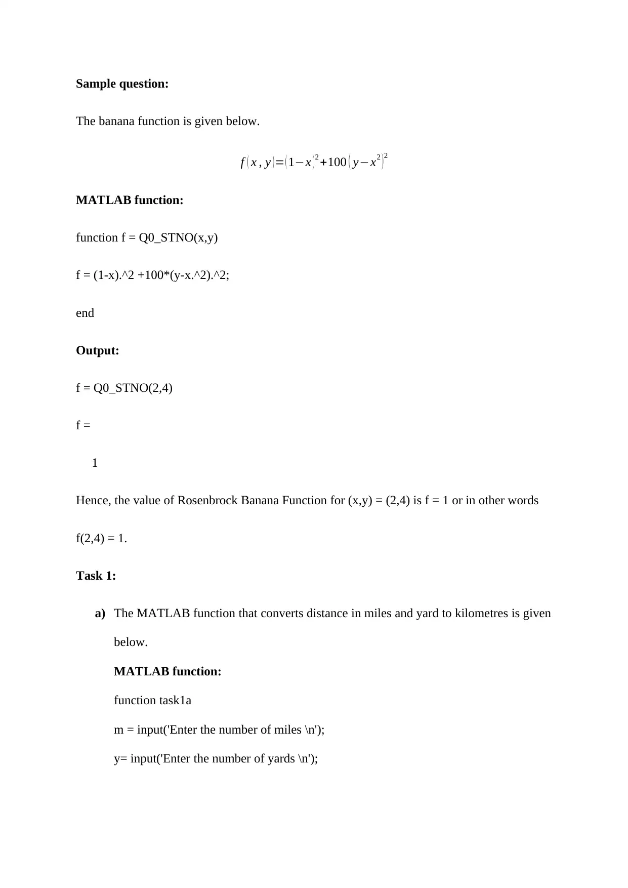
The banana function is given below.
f ( x , y ) = ( 1−x ) 2 +100 ( y−x2 ) 2
MATLAB function:
function f = Q0_STNO(x,y)
f = (1-x).^2 +100*(y-x.^2).^2;
end
Output:
f = Q0_STNO(2,4)
f =
1
Hence, the value of Rosenbrock Banana Function for (x,y) = (2,4) is f = 1 or in other words
f(2,4) = 1.
Task 1:
a) The MATLAB function that converts distance in miles and yard to kilometres is given
below.
MATLAB function:
function task1a
m = input('Enter the number of miles \n');
y= input('Enter the number of yards \n');

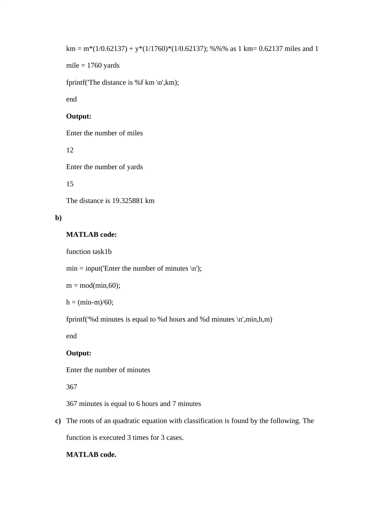
km = m*(1/0.62137) + y*(1/1760)*(1/0.62137); %%% as 1 km= 0.62137 miles and 1
mile = 1760 yards
fprintf('The distance is %f km \n',km);
end
Output:
Enter the number of miles
12
Enter the number of yards
15
The distance is 19.325881 km
b)
MATLAB code:
function task1b
min = input('Enter the number of minutes \n');
m = mod(min,60);
h = (min-m)/60;
fprintf('%d minutes is equal to %d hours and %d minutes \n',min,h,m)
end
Output:
Enter the number of minutes
367
367 minutes is equal to 6 hours and 7 minutes
c) The roots of an quadratic equation with classification is found by the following. The
function is executed 3 times for 3 cases.
MATLAB code.

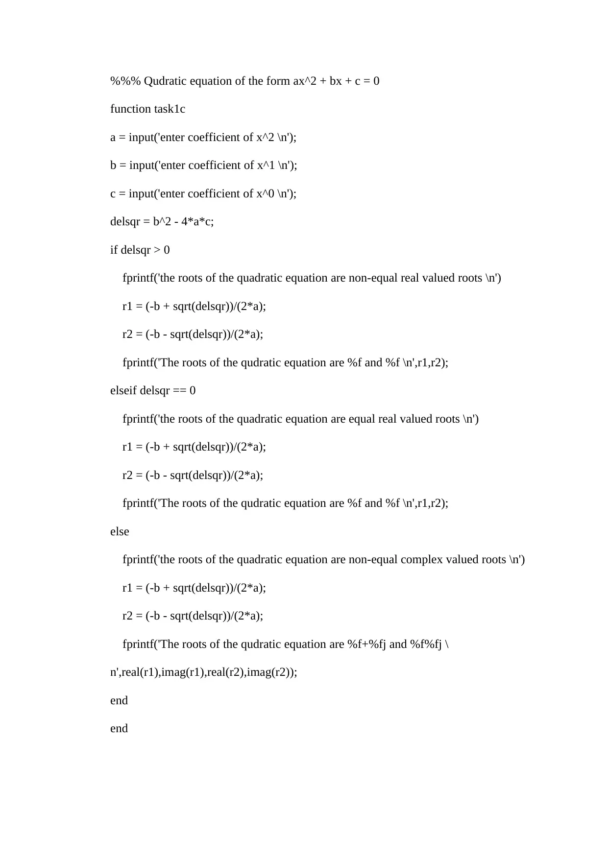
%%% Qudratic equation of the form ax^2 + bx + c = 0
function task1c
a = input('enter coefficient of x^2 \n');
b = input('enter coefficient of x^1 \n');
c = input('enter coefficient of x^0 \n');
delsqr = b^2 - 4*a*c;
if delsqr > 0
fprintf('the roots of the quadratic equation are non-equal real valued roots \n')
r1 = (-b + sqrt(delsqr))/(2*a);
r2 = (-b - sqrt(delsqr))/(2*a);
fprintf('The roots of the qudratic equation are %f and %f \n',r1,r2);
elseif delsqr == 0
fprintf('the roots of the quadratic equation are equal real valued roots \n')
r1 = (-b + sqrt(delsqr))/(2*a);
r2 = (-b - sqrt(delsqr))/(2*a);
fprintf('The roots of the qudratic equation are %f and %f \n',r1,r2);
else
fprintf('the roots of the quadratic equation are non-equal complex valued roots \n')
r1 = (-b + sqrt(delsqr))/(2*a);
r2 = (-b - sqrt(delsqr))/(2*a);
fprintf('The roots of the qudratic equation are %f+%fj and %f%fj \
n',real(r1),imag(r1),real(r2),imag(r2));
end
end

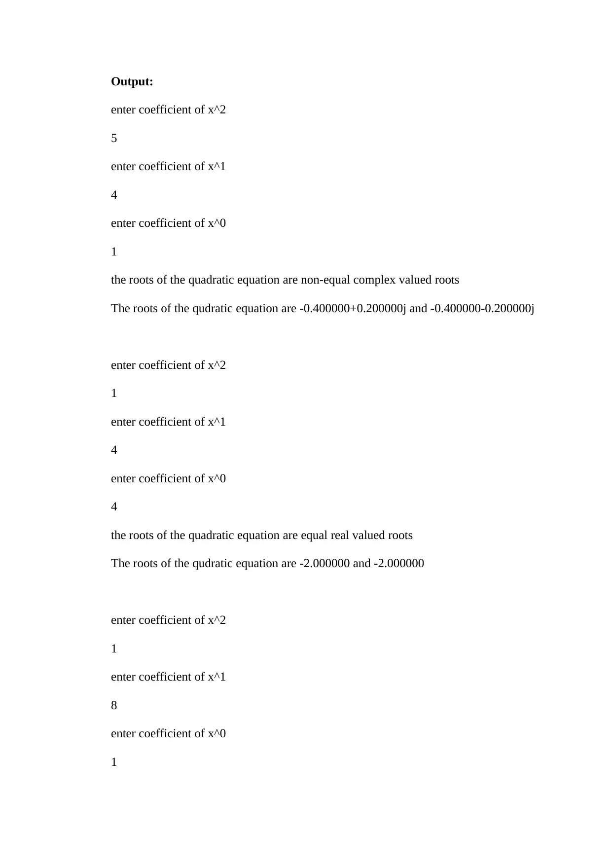
Output:
enter coefficient of x^2
5
enter coefficient of x^1
4
enter coefficient of x^0
1
the roots of the quadratic equation are non-equal complex valued roots
The roots of the qudratic equation are -0.400000+0.200000j and -0.400000-0.200000j
enter coefficient of x^2
1
enter coefficient of x^1
4
enter coefficient of x^0
4
the roots of the quadratic equation are equal real valued roots
The roots of the qudratic equation are -2.000000 and -2.000000
enter coefficient of x^2
1
enter coefficient of x^1
8
enter coefficient of x^0
1

the roots of the quadratic equation are non-equal real valued roots
The roots of the qudratic equation are -0.127017 and -7.872983
Task 2:
In this task the speed(in km/hr) is used as the independent variable and the total
braking distance is used as dependent variable.
Total braking distance = Thinking distance + braking distance = average thinking
time*(speed) + braking distance.
The braking distance (in m) is given for 6 different speeds (km/hr) in the question.
MATLAB code:
speed = [50 70 100 120 145 200]; % speed data
n= length(speed);
brake = [5 12.3 21 32.9 47.6 84.7]; % braking distance data
think = 1.8*(5/18).*speed; % Thinking distance. 1 km/hr = (5/18) m/sec.
tdist = think + brake; % total distance = branking distance + thinking distance
R = (n*sum(tdist.*speed) - sum(tdist)*sum(speed))/sqrt((n*sum(tdist.^2) -
(sum(tdist))^2)*(n*sum(speed.^2) - sum(speed)^2)); %% correleation coeffcient
calculation
a1 = R*((std(tdist)/std(speed))); % a1 = R*(sy/sx)
a0 = mean(tdist) - a1*mean(speed); % a0 = mean(y) - a1*mean(x)
fprintf('The coeffcient a0 = %f, coeffcient a1=%f and coefficient of determination
R^2 = %f \n',a0,a1,R^2)
y = repmat(a0,1,length(speed)) + a1.*speed; % least square regression line y = a0+
a1*x
scatter(speed,tdist)
hold on

plot(speed,y)
title('Scatter plot and fitted regression line')
xlabel('Speed in Km/hr')
ylabel('total braking distance in meters')
Output:
50 100 150 200
Speed in Km/hr
20
40
60
80
100
120
140
160
180
200
total braking distance in meters
Scatter plot and fitted regression line
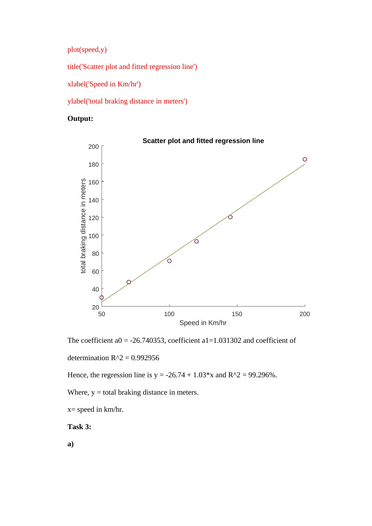
The coefficient a0 = -26.740353, coefficient a1=1.031302 and coefficient of
determination R^2 = 0.992956
Hence, the regression line is y = -26.74 + 1.03*x and R^2 = 99.296%.
Where, y = total braking distance in meters.
x= speed in km/hr.
Task 3:
a)

i) The MATLAB function for calculating the value of sin(π/5) by using its
Taylor series of 1 to 6 terms( i.e. by using n=0 term, sum of n=0 and n=1
terms,…, sum of n=0 to n=5th terms) is given below. Additionally, the
percentage error from the true value of sin(π/5) (calculated using MATLAB
built in sin(x)) for each of the 6 cases is plotted w.r.t number of terms used.
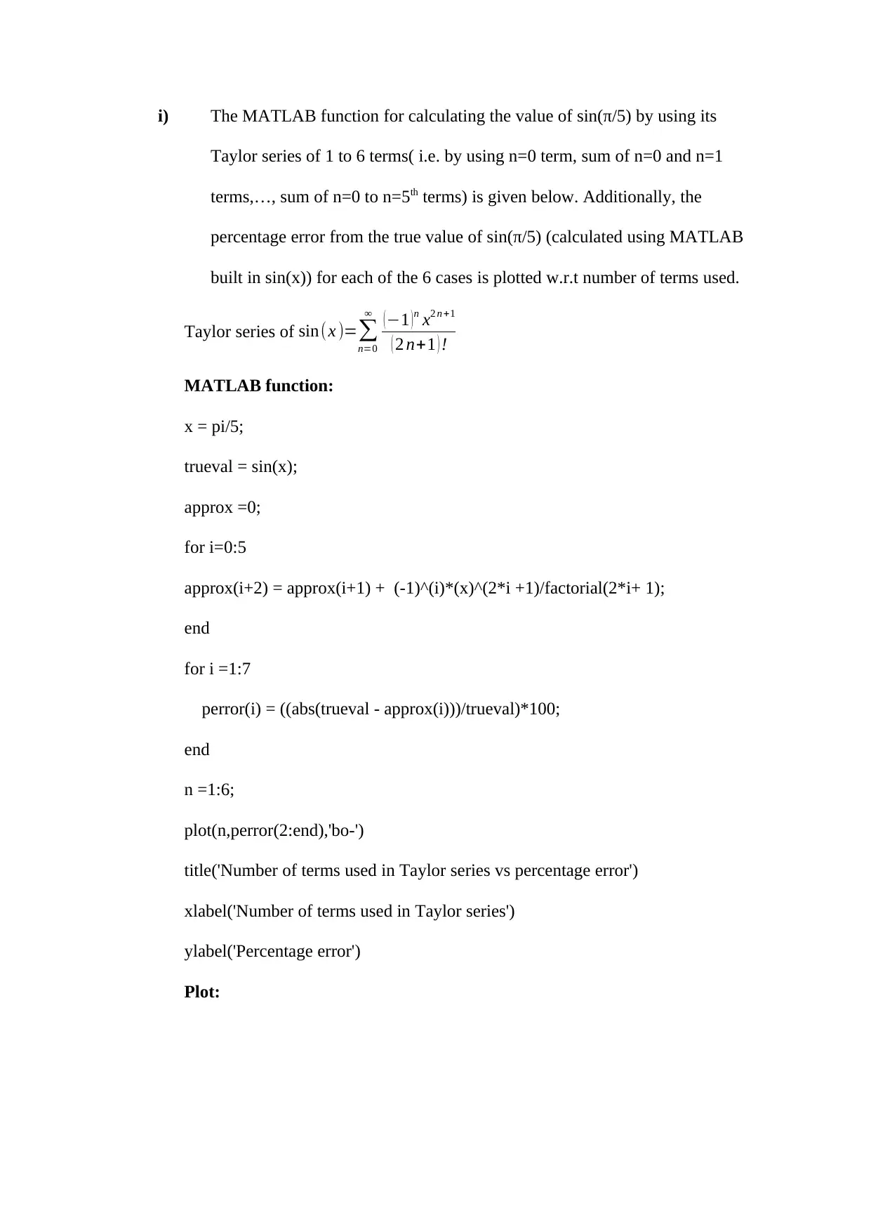
Taylor series of sin(x )=∑
n=0
∞ (−1 )n x2 n +1
( 2 n+1 ) !
MATLAB function:
x = pi/5;
trueval = sin(x);
approx =0;
for i=0:5
approx(i+2) = approx(i+1) + (-1)^(i)*(x)^(2*i +1)/factorial(2*i+ 1);
end
for i =1:7
perror(i) = ((abs(trueval - approx(i)))/trueval)*100;
end
n =1:6;
plot(n,perror(2:end),'bo-')
title('Number of terms used in Taylor series vs percentage error')
xlabel('Number of terms used in Taylor series')
ylabel('Percentage error')
Plot:

1 1.5 2 2.5 3 3.5 4 4.5 5 5.5 6
Number of terms used in Taylor series
0
1
2
3
4
5
6
7
Percentage error
Number of terms used in Taylor series vs percentage error
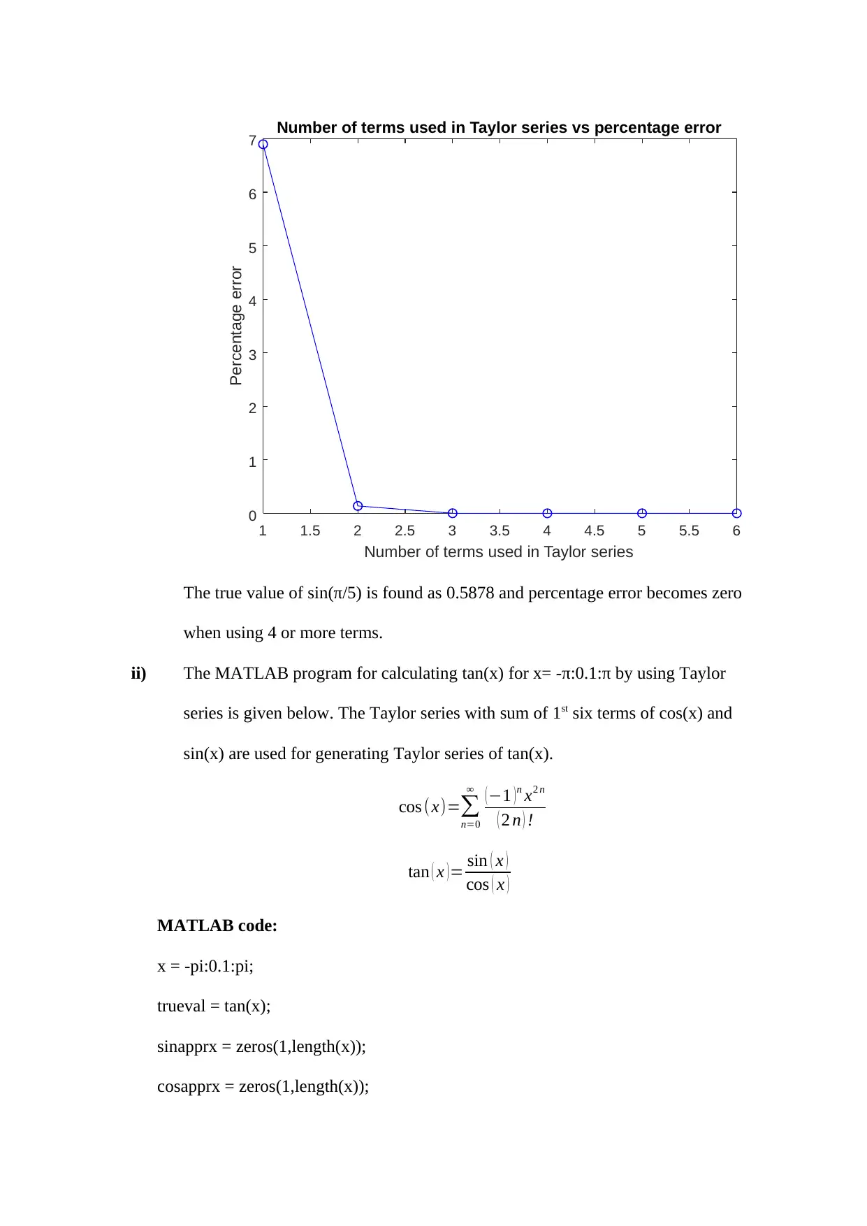
The true value of sin(π/5) is found as 0.5878 and percentage error becomes zero
when using 4 or more terms.
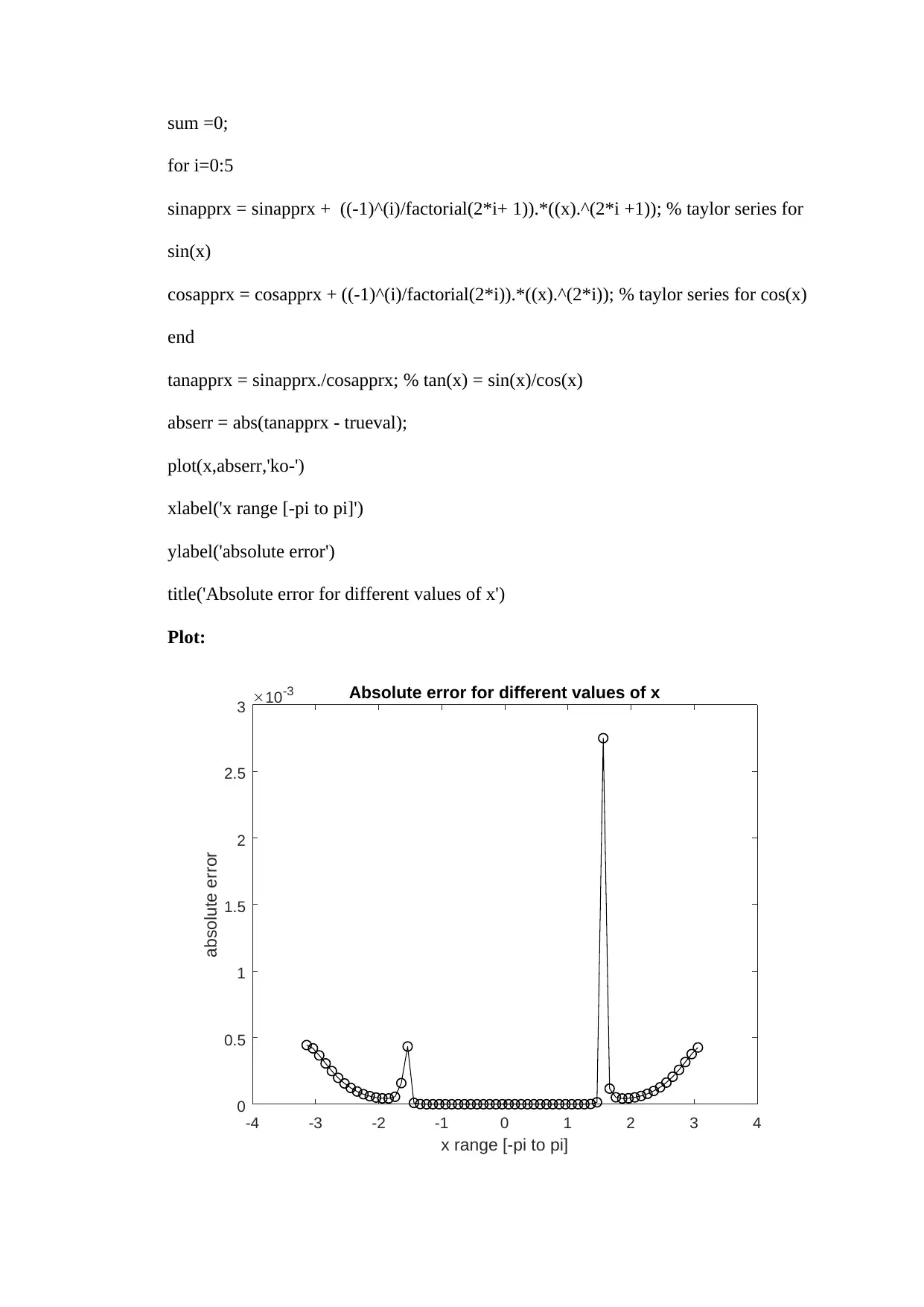
ii) The MATLAB program for calculating tan(x) for x= -π:0.1:π by using Taylor
series is given below. The Taylor series with sum of 1st six terms of cos(x) and
sin(x) are used for generating Taylor series of tan(x).
cos (x)=∑
n=0
∞ (−1 )n x2 n
( 2 n ) !
tan ( x )= sin ( x )
cos ( x )
MATLAB code:
x = -pi:0.1:pi;
trueval = tan(x);
sinapprx = zeros(1,length(x));
cosapprx = zeros(1,length(x));

sum =0;
for i=0:5
sinapprx = sinapprx + ((-1)^(i)/factorial(2*i+ 1)).*((x).^(2*i +1)); % taylor series for
sin(x)
cosapprx = cosapprx + ((-1)^(i)/factorial(2*i)).*((x).^(2*i)); % taylor series for cos(x)
end
tanapprx = sinapprx./cosapprx; % tan(x) = sin(x)/cos(x)
abserr = abs(tanapprx - trueval);
plot(x,abserr,'ko-')
xlabel('x range [-pi to pi]')
ylabel('absolute error')
title('Absolute error for different values of x')
Plot:
-4 -3 -2 -1 0 1 2 3 4
x range [-pi to pi]
0
0.5
1
1.5
2
2.5
3
absolute error
10-3 Absolute error for different values of x

b) Now, a MATLAB program is developed which can determine the value of n i.e.
the number of terms used in Taylor series of sin(x) (x= -π:0.1:π) such that the
truncation error is always below some specified threshold limit. The minimum
value of n and average of truncation error and maximum of truncation error for
that n is also displayed. The user input of threshold limit in this case is 10^(-4).
MATLAB function:
function task3b(value)
x = -pi:0.1:pi;
trueval = sin(x);
approx =zeros(1,length(x));
n=0; threshold = abs(approx-trueval); value=repmat(value,1,length(threshold));
for j=1:length(threshold)
while threshold(j) >= value(j)
approx = approx + ((-1)^(n)/factorial(2*n+ 1)).*((x).^(2*n +1));
n=n+1;
threshold = abs(trueval-approx);
end
end
fprintf('The minimum n value is %d \nThe average truncation error is %f \nThe
maximum truncation error is %f \n',n,mean(threshold),max(threshold))
end

Output:
task3b(1e-4)
The minimum n value is 7
The average truncation error is 0.000001
The maximum truncation error is 0.000021