MATLAB Homework: Intracranial Pressure and EOG Signal Analysis

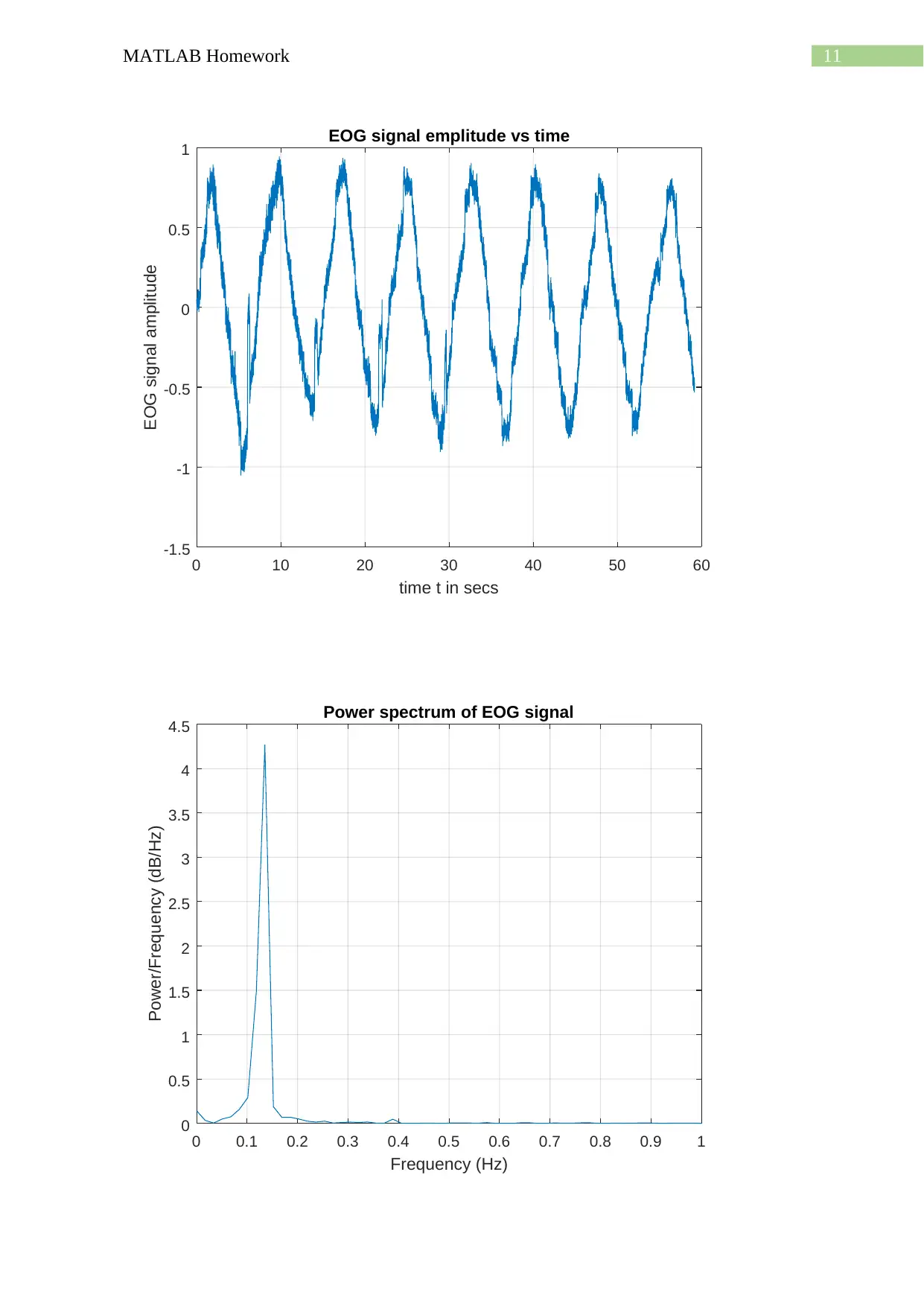
This MATLAB homework assignment addresses two main problems. The first involves analyzing a system's response to different input injections, modeling intracranial pressure using a transfer function, and calculating compliance. The solution includes MATLAB code to simulate the system's behavior, generate plots for varying injection volumes, and calculate compliance values. The second problem focuses on processing an electrooculogram (EOG) signal. The solution involves loading EOG data, calculating statistical properties like mean and power, and performing a Fourier transform to analyze the signal's frequency spectrum. The provided MATLAB code calculates the mean, power, and power spectral density of the EOG signal, along with the frequency at which maximum power occurs, providing a comprehensive analysis of the signal's characteristics and the system parameters.

Running head: MATLAB Homework
MATLAB Homework
Name of the Student
Name of the University
Author Note

1MATLAB Homework
9.1:
Given, input-output equation is
τdΔP ( t )
dt + ΔP ( t ) =kr ( t )
Now, taking Laplace transform of the equation we get,
τ s ΔP ( s ) + ΔP ( s ) =k∗R (s)
=> ΔP ( s )
R ( s ) = k
τs+1
a) Now, from the figure 31 given that,
For ΔV = 0.1,0.2,0.3 and 0.4 mL injection is on ton = 15 secs and stays for 2,4,6 and 8 secs
respectively. The amplitude of signal r(t) = 0.05 mL/sec or 5 mmHg.
MATLAB code:
t = 0:1:180;
k = 55; tao = 66;P0 = 0.12; % Assuming system parameters
sys = tf(k,[tao,1]); % transfer function
%% delV = 0.1 mL or injection time = 2 secs.
r = zeros(1,length(t));
r(16:18) = 0.05;
P = lsim(sys,r,t); P = P + P0;

2MATLAB Homework
figure(1)
plot(t,P,'b-')
hold on
plot(t,r,'r-')
xlabel('Time in sec')
ylabel('Intracranial pressure in mmHg')
title('P(t) vs t and r(t) vs t')
grid on
legend('P(t)','r(t)')
hold off
%% delV = 0.2 mL or injection time = 4 secs.
r = zeros(1,length(t));
r(16:20) = 0.05;
P = lsim(sys,r,t); P = P + P0;
figure(2)
plot(t,P)
hold on
plot(t,r)

3MATLAB Homework
xlabel('Time in sec')
ylabel('Intracranial pressure in mmHg')
title('P(t) vs t and r(t) vs t')
legend('P(t)','r(t)')
grid on
hold off
%% delV = 0.3 mL or injection time = 6 secs.
r = zeros(1,length(t));
r(16:22) = 0.05;
P = lsim(sys,r,t); P = P + P0;
figure(3)
plot(t,P)
hold on
plot(t,r)
xlabel('Time in sec')
ylabel('Intracranial pressure in mmHg')
title('P(t) vs t and r(t) vs t')
grid on

4MATLAB Homework
legend('P(t)','r(t)')
hold off
%% delV = 0.4 mL or injection time = 8 secs.
r = zeros(1,length(t));
r(16:24) = 0.05;
P = lsim(sys,r,t); P = P + P0;
figure(4)
plot(t,P)
hold on
plot(t,r)
xlabel('Time in sec')
ylabel('Intracranial pressure in mmHg')
title('P(t) vs t and r(t) vs t')
grid on
legend('P(t)','r(t)')
hold off

5MATLAB Homework
Outputs:
ΔV = 0.1 mL
0 20 40 60 80 100 120 140 160 180
Time in sec
0
0.05
0.1
0.15
0.2
0.25
mL/sec
P(t) vs t and r(t) vs t
P(t)
r(t)
ΔV = 0.2 mL:

6MATLAB Homework
0 20 40 60 80 100 120 140 160 180
Time in sec
0
0.05
0.1
0.15
0.2
0.25
0.3
0.35
mL/sec
P(t) vs t and r(t) vs t
P(t)
r(t)
ΔV = 0.3 mL:
0 20 40 60 80 100 120 140 160 180
Time in sec
0
0.05
0.1
0.15
0.2
0.25
0.3
0.35
0.4
mL/sec
P(t) vs t and r(t) vs t
P(t)
r(t)

7MATLAB Homework
ΔV = 0.4 mL:
0 20 40 60 80 100 120 140 160 180
Time in sec
0
0.05
0.1
0.15
0.2
0.25
0.3
0.35
0.4
0.45
0.5
mL/sec
P(t) vs t and r(t) vs t
P(t)
r(t)
b) Hence, as seen from the above plots that the optimum parameters of the system are k = 55,
τ = 66 and P0 = 0.12 mL/sec which produces closest plots like given in Figure 31 in question
for different ΔV.
c) Now, for each ΔV the differential pressure ΔP is calculated is given by the following
formula.
ΔP = Max{P(t)} – P0;
Then compliance C is calculated by,
C = ΔV/ΔP.
MATLAB code:
delP = max(P) - P0;

8MATLAB Homework
delv = 0.1;
C = delv/delP;
fprintf('At delV =%.1f mL delP = %.2f mL/sec and Compliance C = %.2f mL/mmHg\
n',delv,delP,C)
delP = max(P) - P0;
delv = 0.2;
C = delv/delP;
fprintf('At delV =%.1f mL delP = %.2f mL/sec and Compliance C = %.2f mL/mmHg\
n',delv,delP,C)
delP = max(P) - P0;
delv = 0.3;
C = delv/delP;
fprintf('At delV =%.1f mL delP = %.2f mL/sec and Compliance C = %.2f mL/mmHg\
n',delv,delP,C)
delP = max(P) - P0;
delv = 0.4;
C = delv/delP;
fprintf('At delV =%.1f mL delP = %.2f mL/sec and Compliance C = %.2f mL/mmHg\
n',delv,delP,C)
Output:
At delV =0.1 mL delP = 0.12 mL/sec and Compliance C = 0.82 mL/mmHg

9MATLAB Homework
At delV =0.2 mL delP = 0.20 mL/sec and Compliance C = 1.00 mL/mmHg
At delV =0.3 mL delP = 0.28 mL/sec and Compliance C = 1.08 mL/mmHg
At delV =0.4 mL delP = 0.35 mL/sec and Compliance C = 1.14 mL/mmHg
Hence, it can be seen that the compliance C is largest when ΔV =0.4 mL.
9.2:
MATLAB code:
load('eog_trimmed.mat');
figure(1)
plot(t,eog)
xlabel('time t in secs')
ylabel('EOG signal amplitude')
grid on
title('EOG signal emplitude vs time')
meaneog = mean(eog);
poweog = (1/length(eog))*sum((eog - meaneog).^2);
fprintf('Mean value of EOG signal is %.4f V\n',meaneog)
fprintf('Power of the EOG signal is %.4f V^2\n',poweog)
fs = 1/(t(2)-t(1)); % calculating sampling rate
eogdft = fft(eog); N = length(eog); % number of data point in EOG signal
psdeog = (1/(fs*N))*abs(eogdft).^2; % power spectral density of eog signal

10MATLAB Homework
freq = 0:(fs/N):fs;freq = freq(1:length(freq)-1); % frequency range
figure(2)
plot(freq,psdeog)
xlabel('Frequency (Hz)')
ylabel('Power/Frequency (dB/Hz)')
set(gca,'Xlim',[0,1])
grid on
title('Power spectrum of EOG signal')
Outputs:
Mean value of EOG signal is 0.0492 V
Power of the EOG signal is 0.2398 V^2
The maximum frequency at which the power spectrum of the EOG reaches its maximum
value is fmax = 0.1352 Hz.

11MATLAB Homework
0 10 20 30 40 50 60
time t in secs
-1.5
-1
-0.5
0
0.5
1
EOG signal amplitude
EOG signal emplitude vs time
0 0.1 0.2 0.3 0.4 0.5 0.6 0.7 0.8 0.9 1
Frequency (Hz)
0
0.5
1
1.5
2
2.5
3
3.5
4
4.5
Power/Frequency (dB/Hz)
Power spectrum of EOG signal