MATLAB Interpolation, Curve Fitting, and Optimization Problems
VerifiedAdded on 2023/05/28
|56
|6920
|97
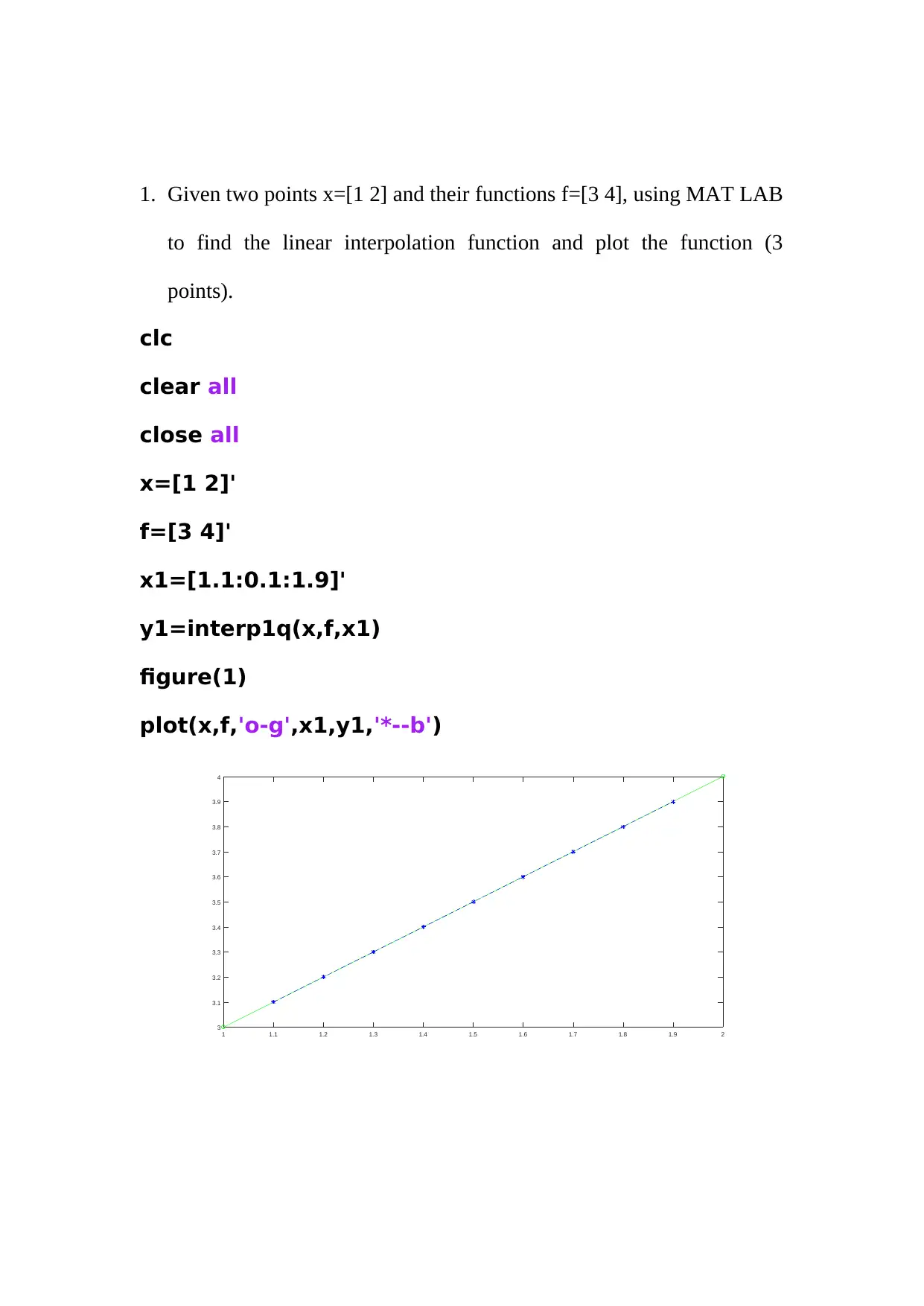
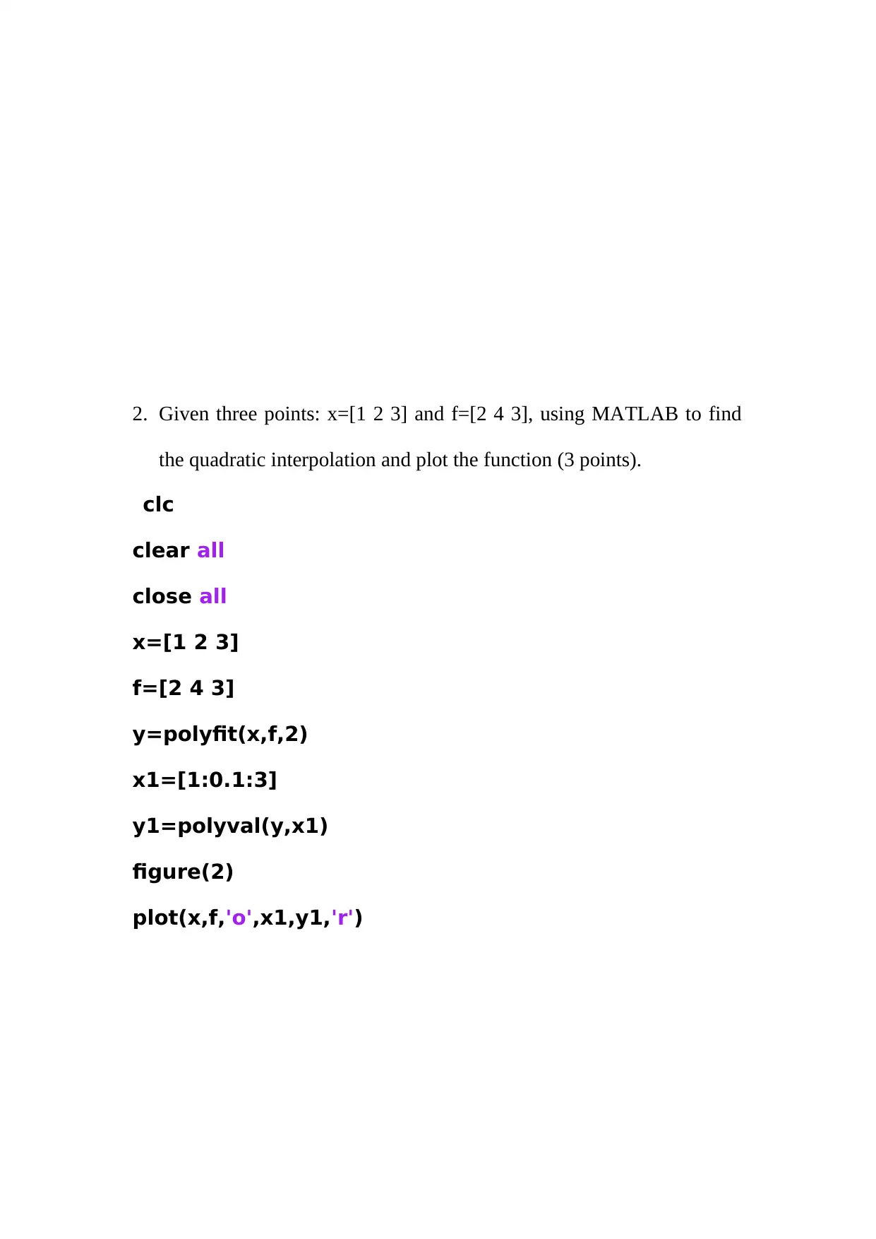
Homework Assignment
AI Summary
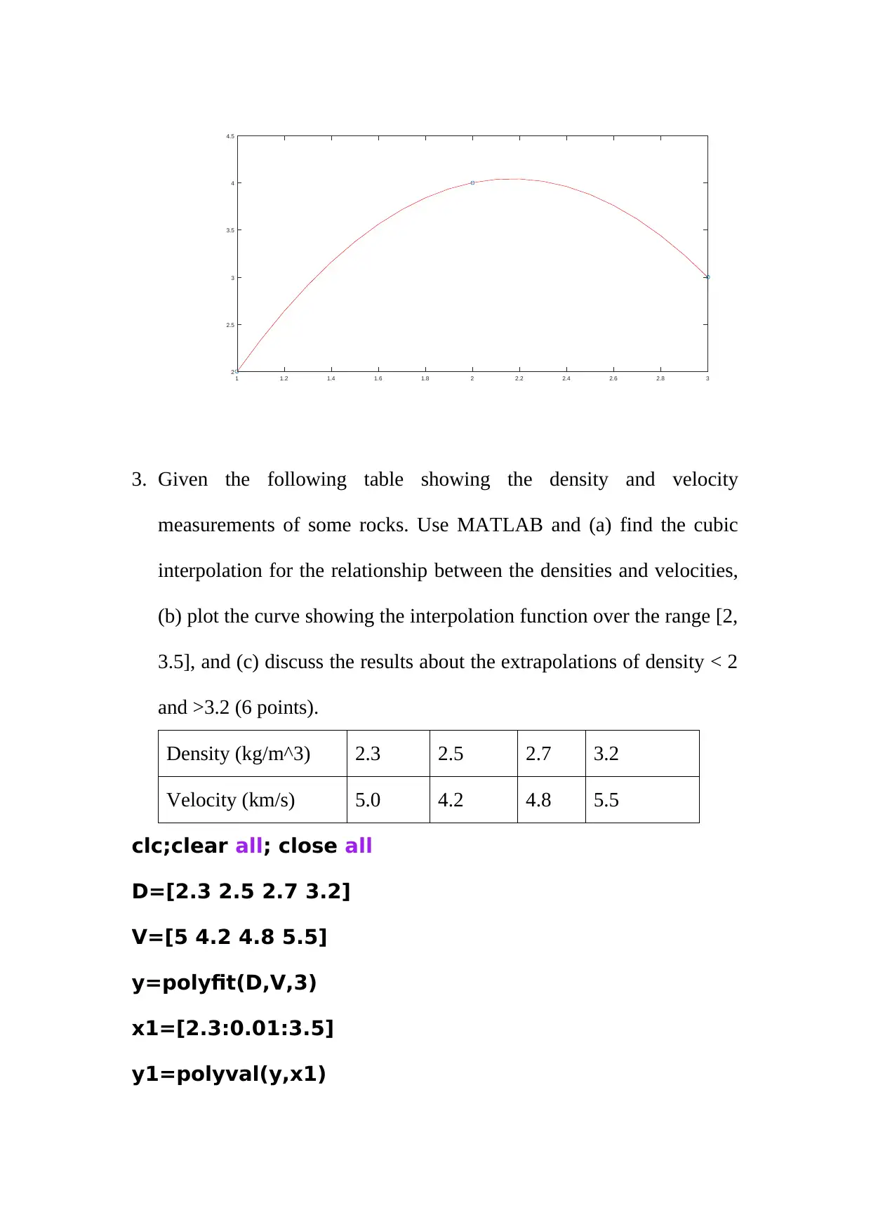
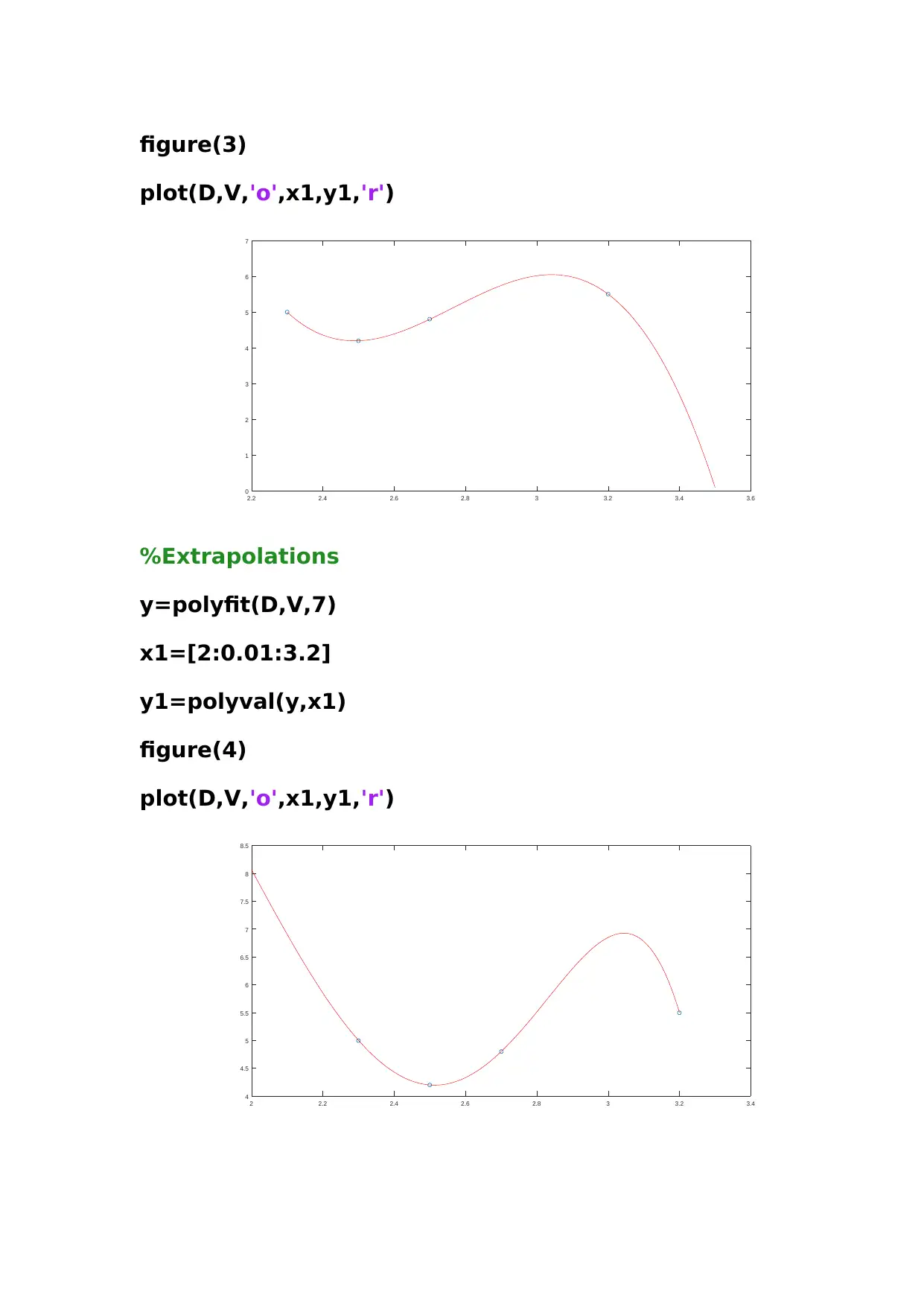
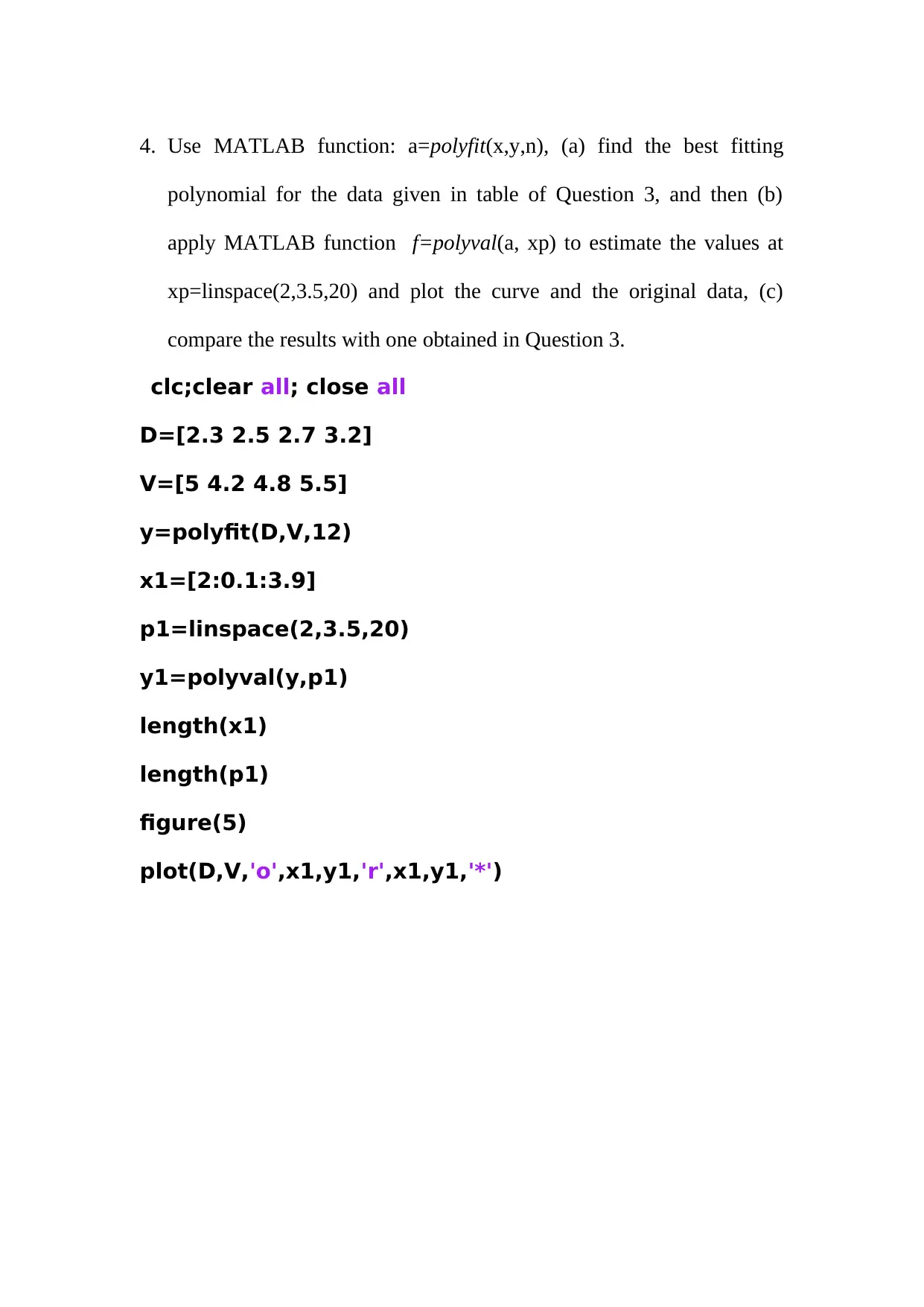
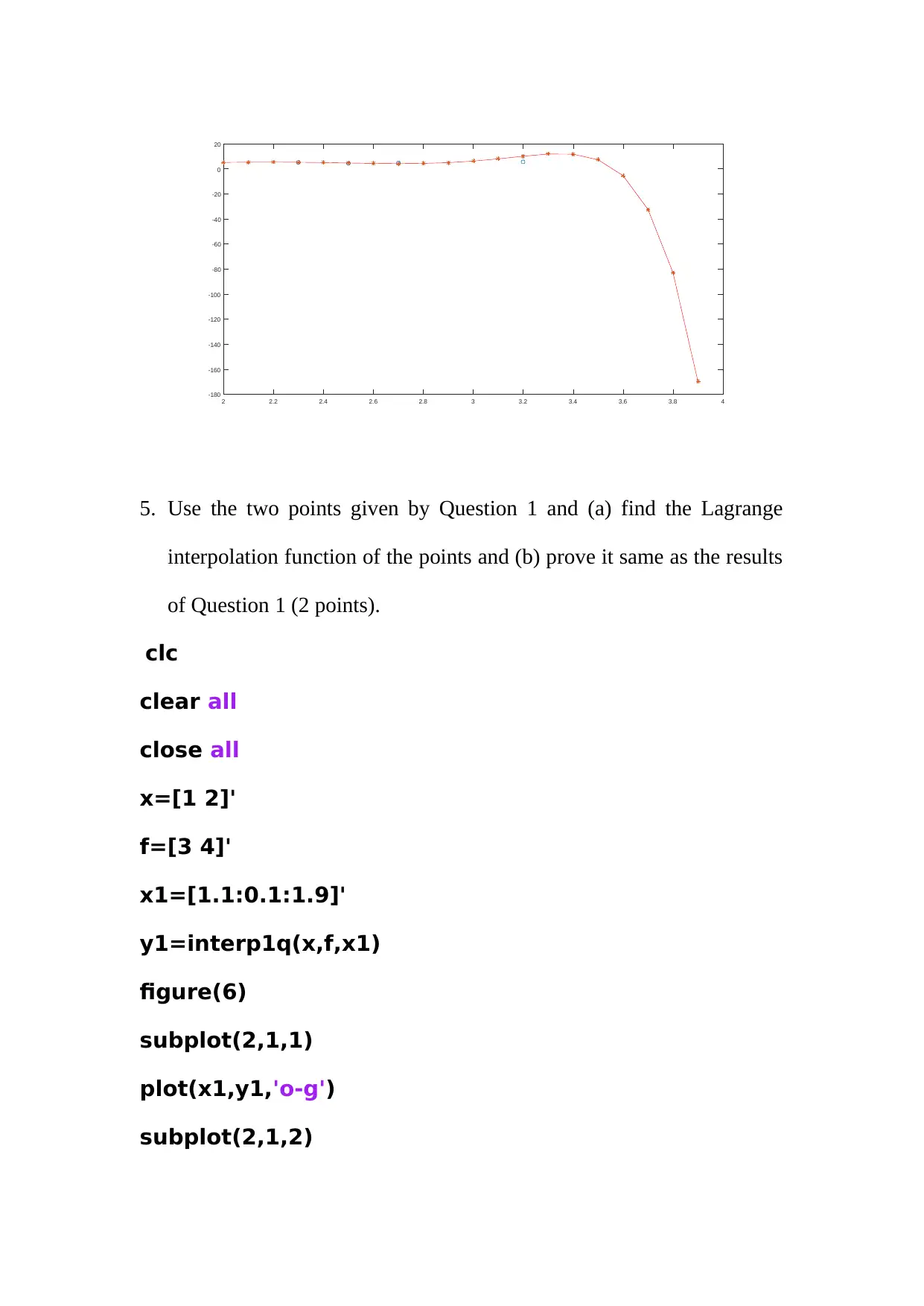
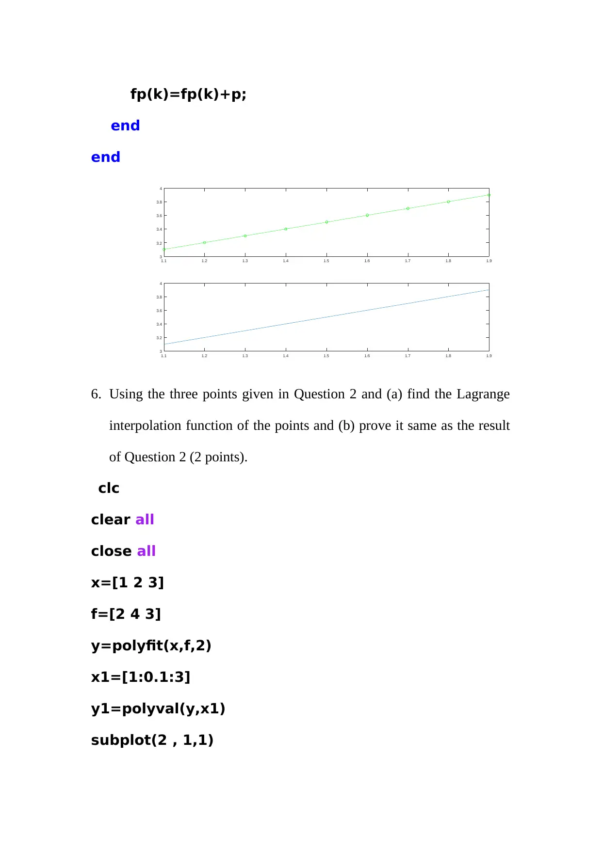
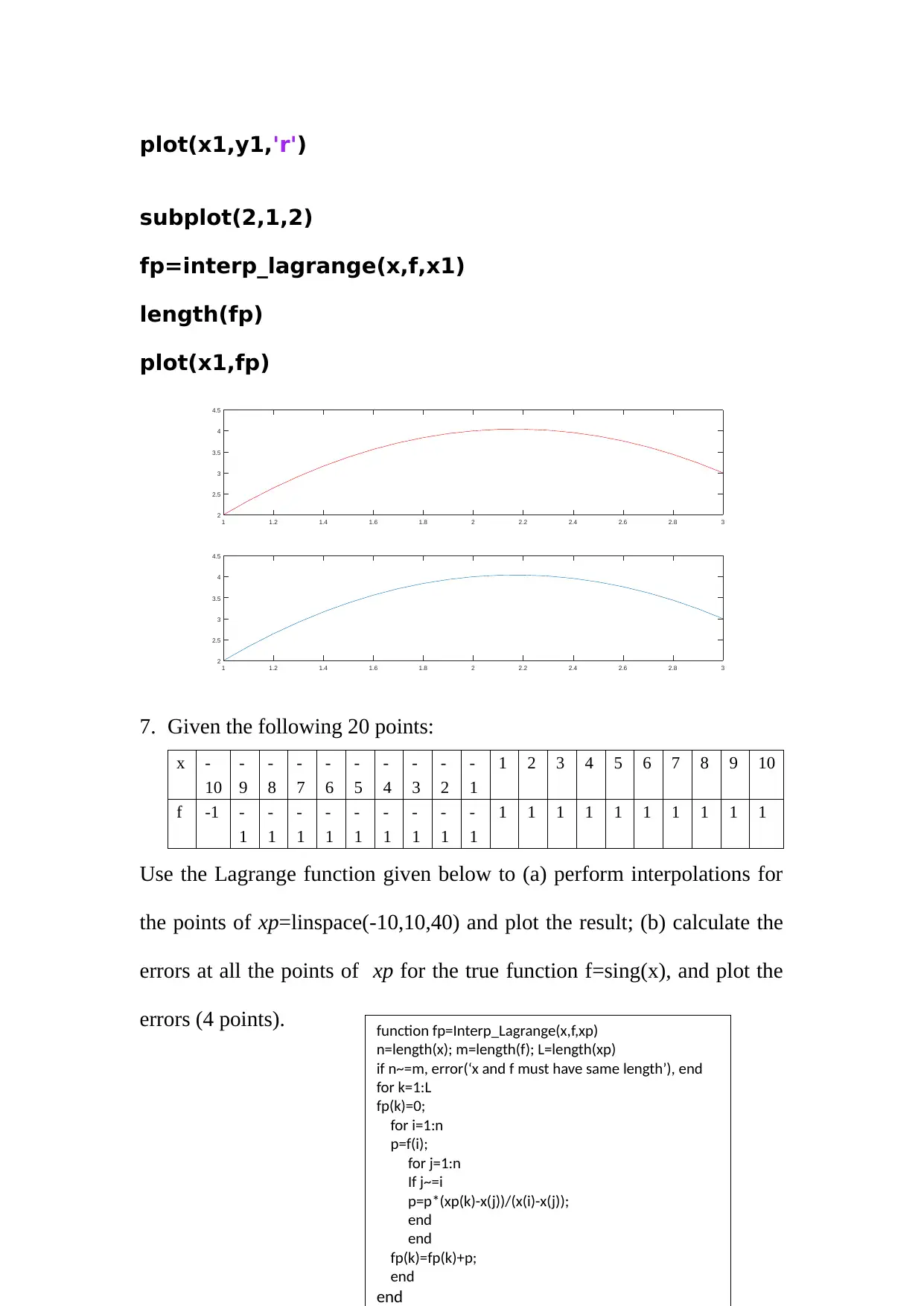
This assignment explores various interpolation techniques, curve fitting, and optimization methods using MATLAB. The solution begins with linear and quadratic interpolation using given points and their corresponding function values. It then delves into cubic interpolation applied to density and velocity measurements, including discussions on extrapolation. The assignment further utilizes MATLAB's polyfit and polyval functions to find the best-fitting polynomials and estimate values, comparing the results with cubic interpolation. Lagrange interpolation is implemented and compared to the initial interpolation results. Additionally, the assignment covers Chebyshev interpolation and its error analysis, followed by a comparison with Lagrange interpolation. The document also includes explanations of polynomial and Lagrange interpolation, as well as spline interpolation. Furthermore, it addresses the concepts of minima, maxima, and optimization, including the application of the bisection method to find the root of a function and the use of MATLAB to find the optimum of a given function. Finally, it discusses the relationships between derivatives and the nature of maxima and minima.


1 out of 56


Your All-in-One AI-Powered Toolkit for Academic Success.
+13062052269
info@desklib.com
Available 24*7 on WhatsApp / Email
![[object Object]](/_next/static/media/star-bottom.7253800d.svg)
Copyright © 2020–2026 A2Z Services. All Rights Reserved. Developed and managed by ZUCOL.