EE472 Lab Report: Modeling Dynamic Systems in Matlab and Simulink

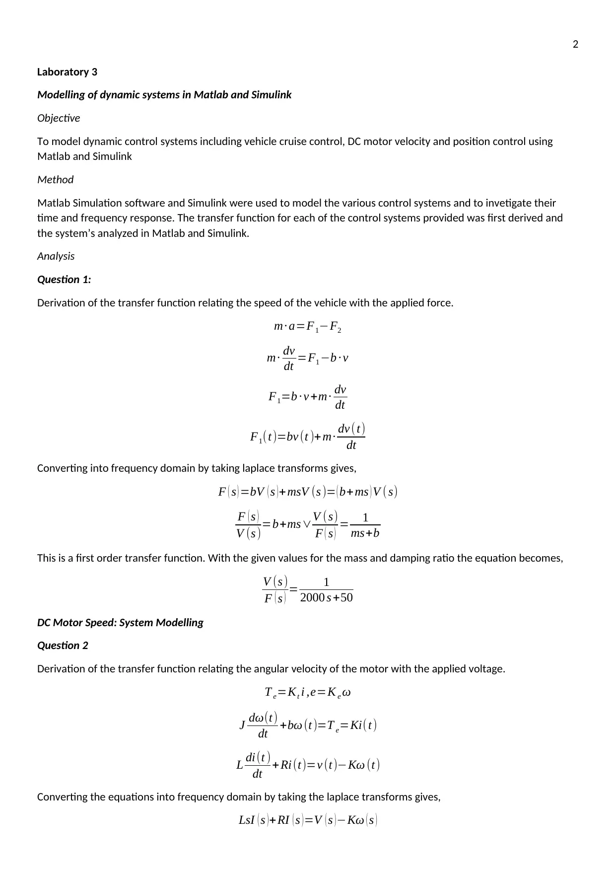
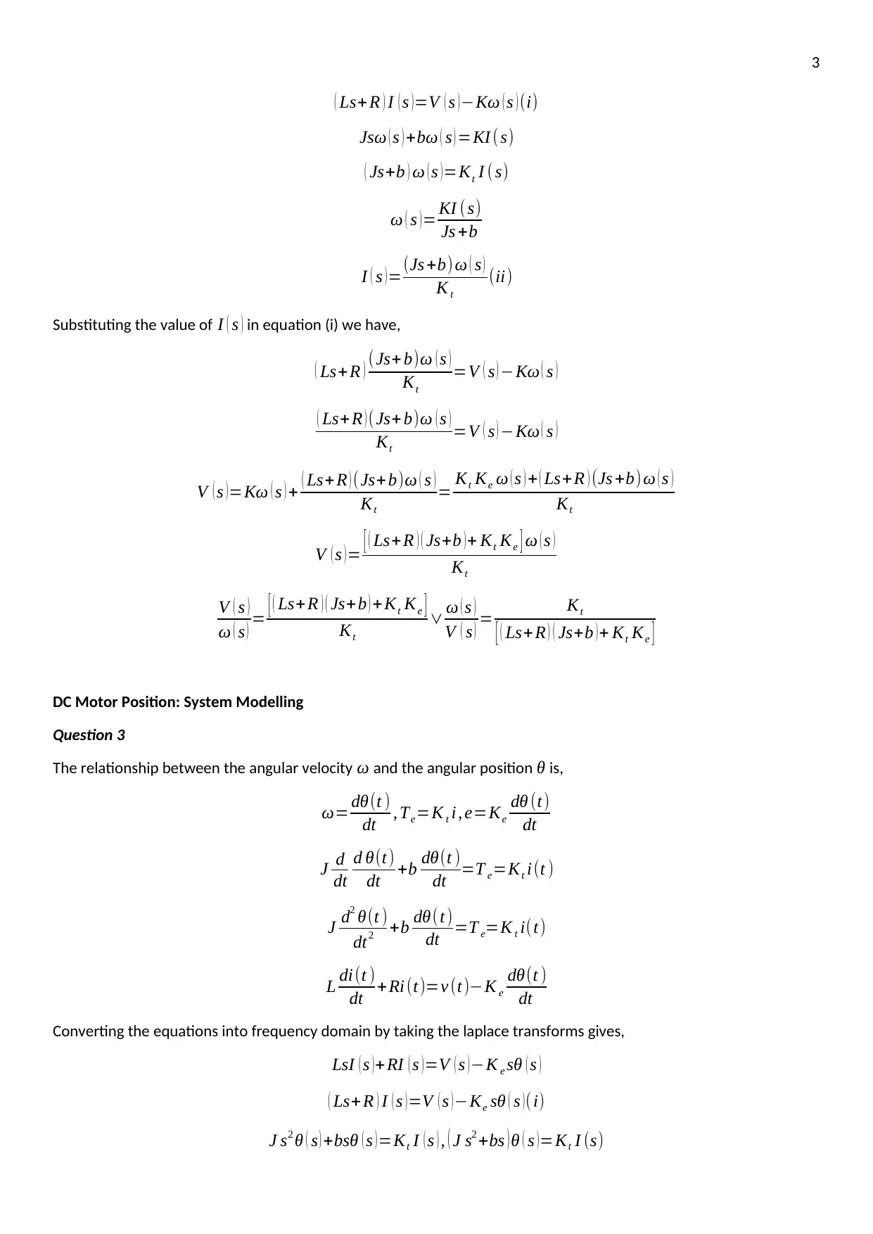
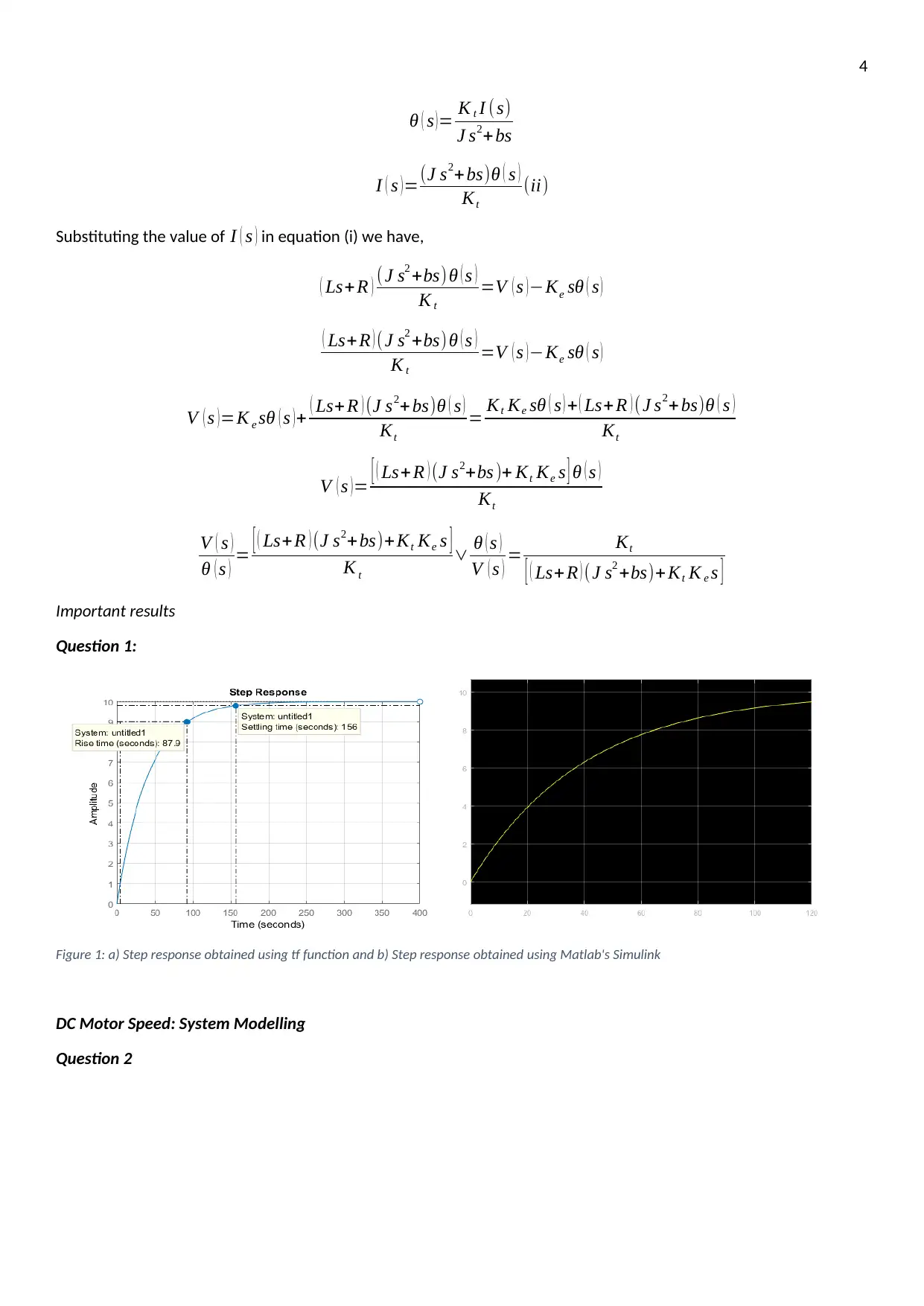
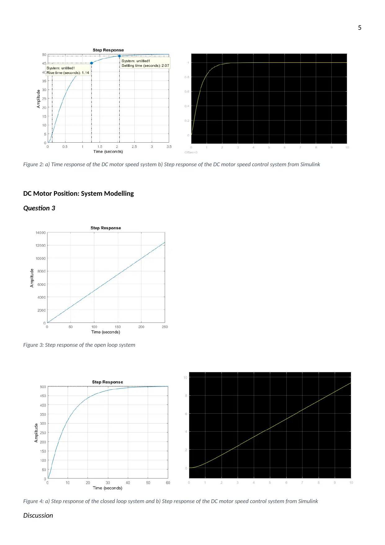
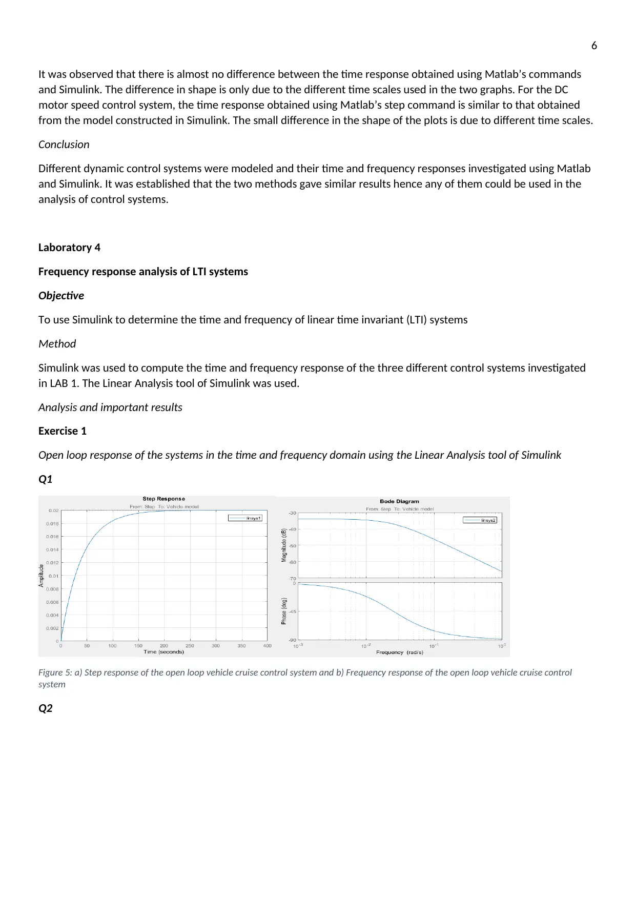
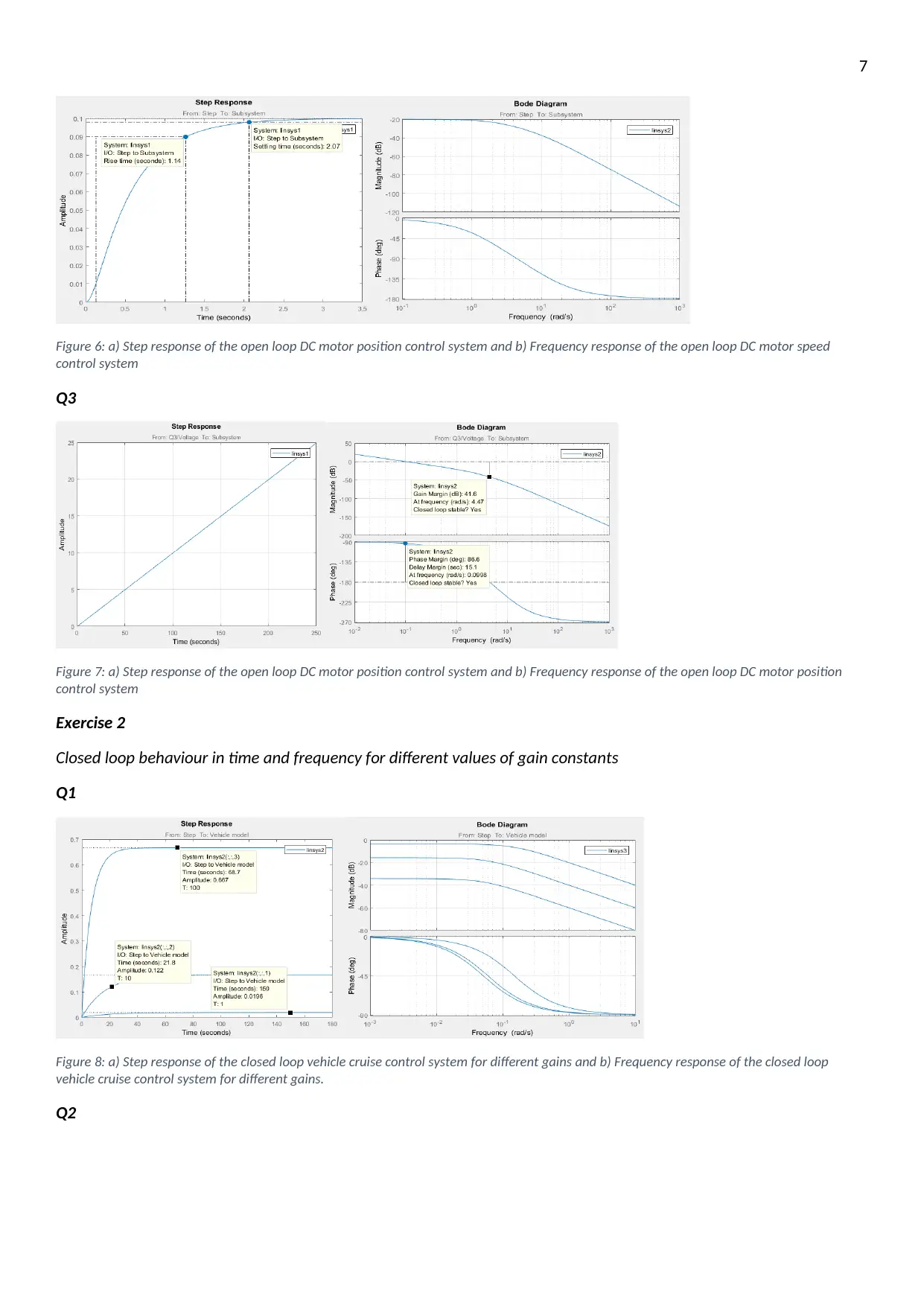
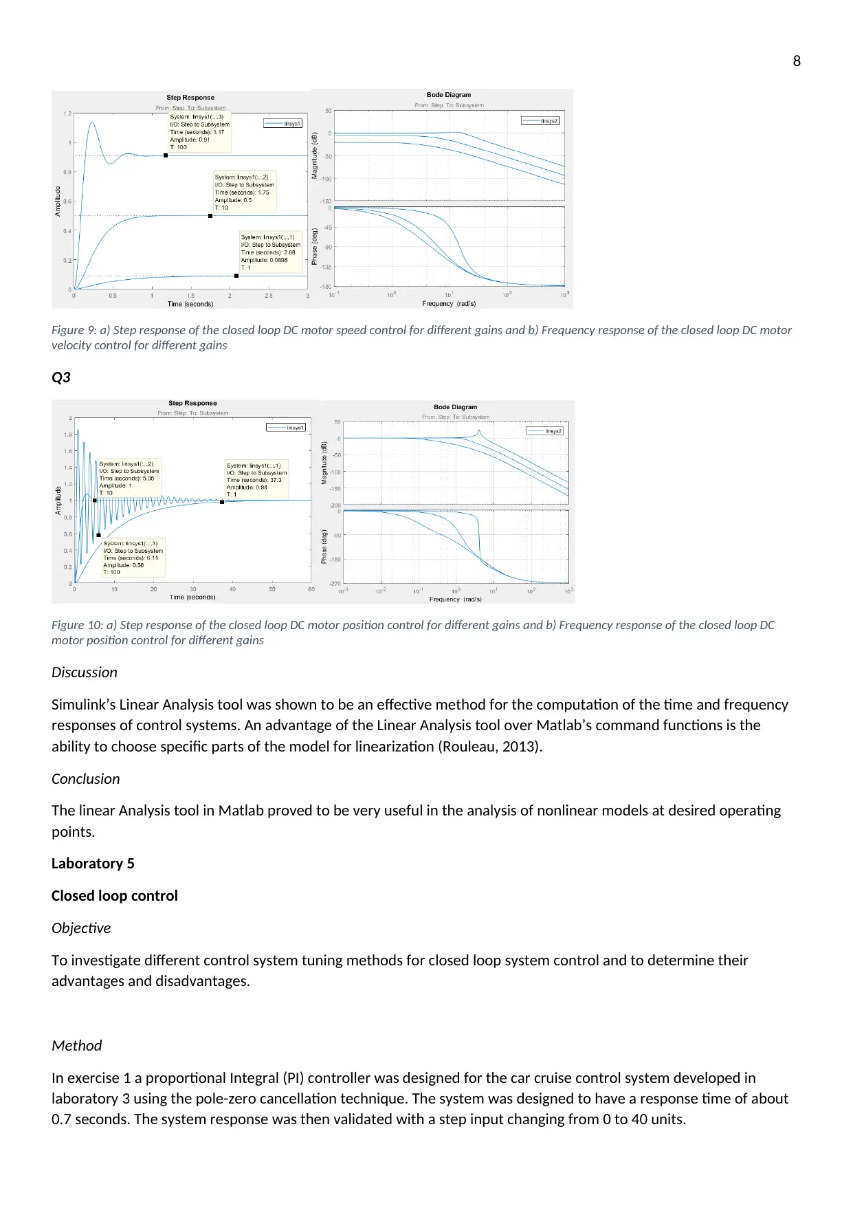
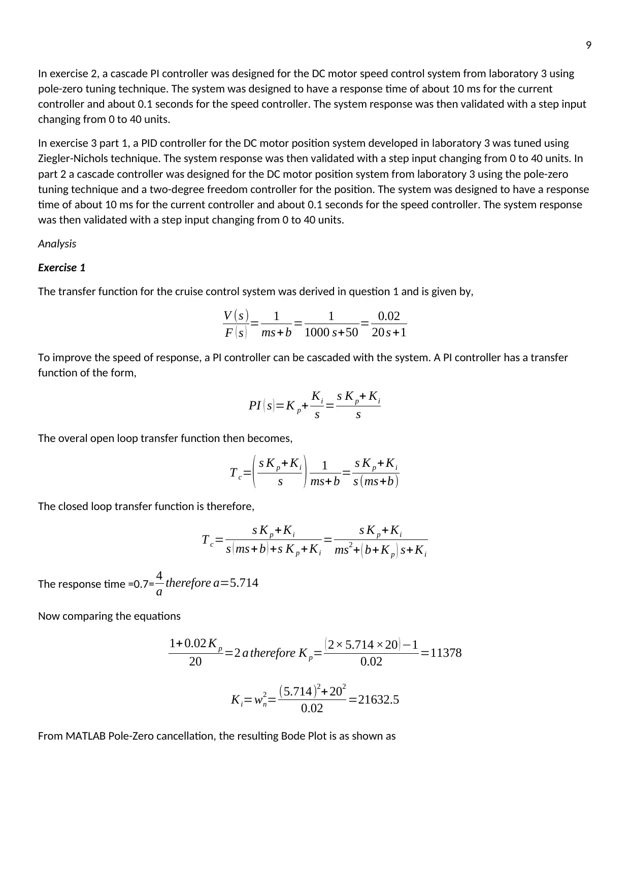
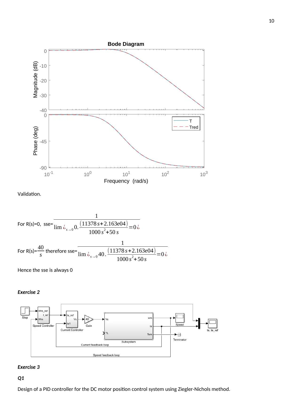
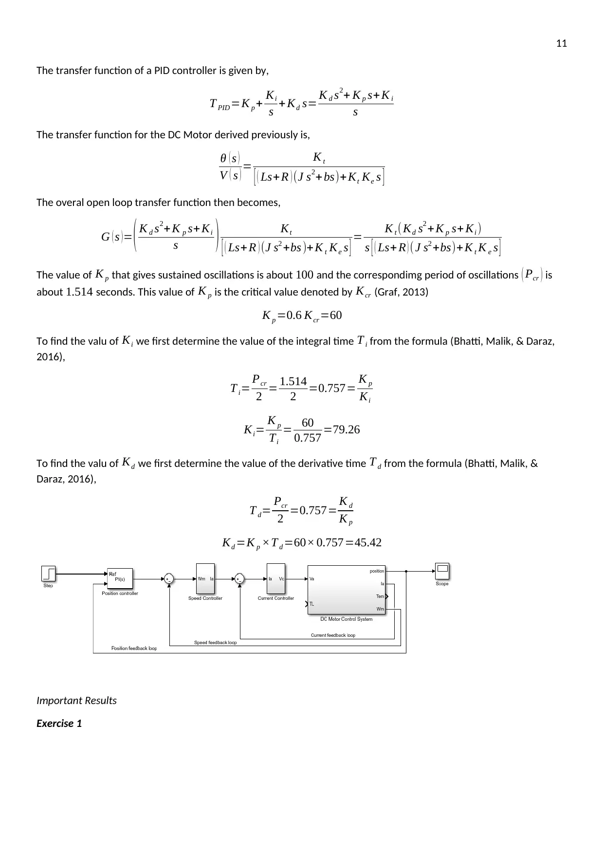
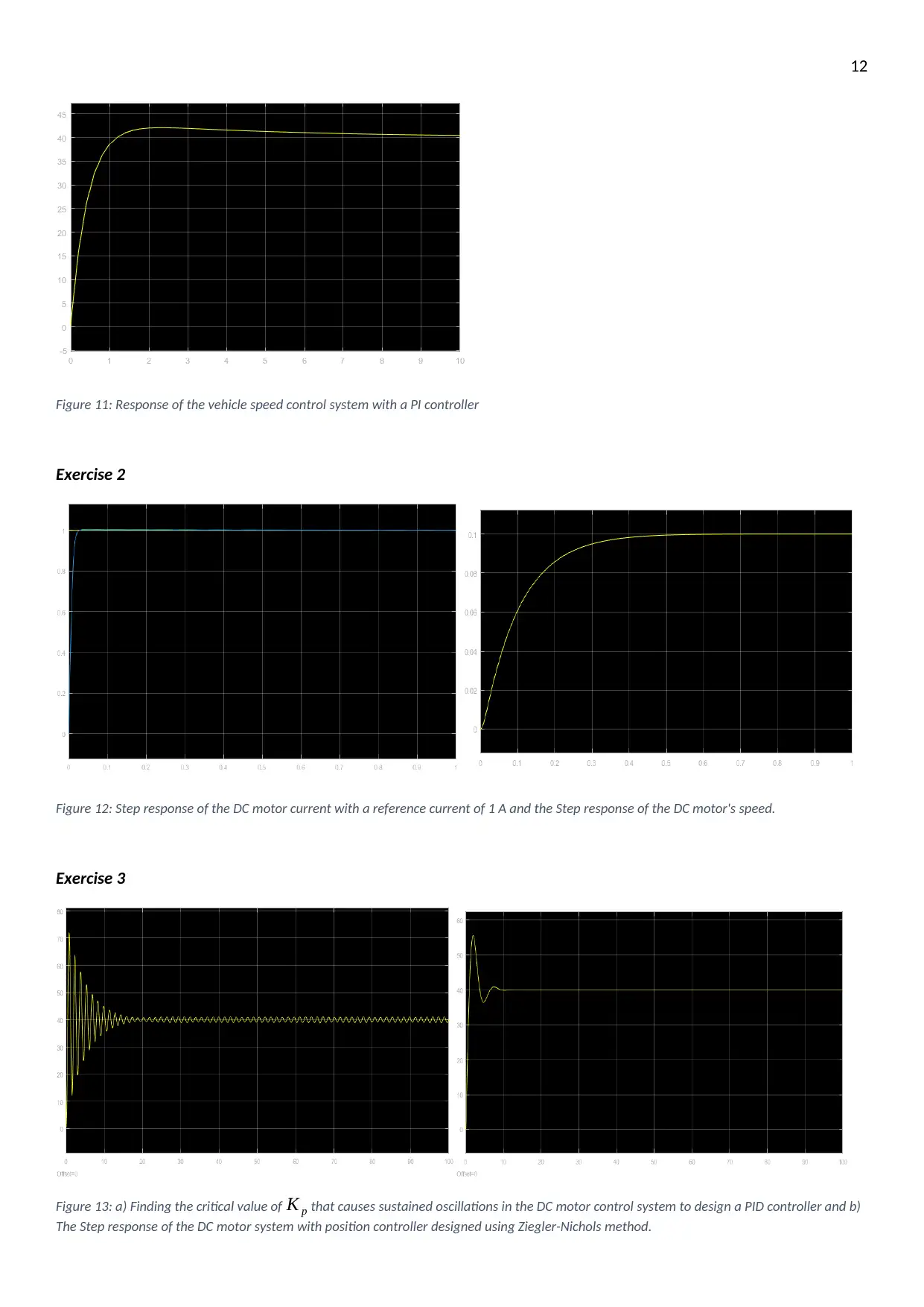
This report details the modeling and analysis of dynamic control systems using Matlab and Simulink. The report covers three laboratory sessions, each focusing on different aspects of control system design and analysis. Laboratory 3 focuses on modeling dynamic systems, including vehicle cruise control and DC motor velocity and position control, deriving transfer functions, and investigating time and frequency responses. Laboratory 4 delves into frequency response analysis of linear time-invariant (LTI) systems using Simulink's Linear Analysis tool. Finally, Laboratory 5 investigates closed-loop control, exploring different control system tuning methods, including PI and PID controllers, and their advantages and disadvantages, using techniques such as pole-zero cancellation and Ziegler-Nichols methods. The report includes derivations, simulations, results, discussions, and conclusions for each lab, providing a comprehensive overview of control system design and analysis techniques.

1
A Joint Laboratory Report
Student’s Name
Institutional Affiliation
Date

2
Laboratory 3
Modelling of dynamic systems in Matlab and Simulink
Objective
To model dynamic control systems including vehicle cruise control, DC motor velocity and position control using
Matlab and Simulink
Method
Matlab Simulation software and Simulink were used to model the various control systems and to invetigate their
time and frequency response. The transfer function for each of the control systems provided was first derived and
the system’s analyzed in Matlab and Simulink.
Analysis
Question 1:
Derivation of the transfer function relating the speed of the vehicle with the applied force.
m∙ a=F1−F2
m∙ dv
dt =F1 −b ∙ v
F1=b ∙ v +m∙ dv
dt
F1(t)=bv (t )+ m∙ dv ( t)
dt
Converting into frequency domain by taking laplace transforms gives,
F ( s ) =bV ( s ) +msV (s )= ( b+ms ) V ( s)
F ( s )
V (s )=b+ms∨V (s)
F ( s ) = 1
ms+b
This is a first order transfer function. With the given values for the mass and damping ratio the equation becomes,
V (s )
F ( s ) = 1
2000 s +50
DC Motor Speed: System Modelling
Question 2
Derivation of the transfer function relating the angular velocity of the motor with the applied voltage.
T e=Kt i ,e=K e ω
J dω(t)
dt +bω (t )=T e=Ki( t)
L di(t )
dt + Ri (t)=v (t)−Kω (t)
Converting the equations into frequency domain by taking the laplace transforms gives,
LsI ( s )+ RI ( s )=V ( s )−Kω ( s )

3
( Ls+ R ) I ( s ) =V ( s ) −Kω ( s ) (i)
Jsω ( s ) +bω ( s ) =KI (s)
( Js+b ) ω ( s )=Kt I ( s)
ω ( s )= KI (s)
Js +b
I ( s )=(Js +b) ω ( s )
K t
(ii)
Substituting the value of I ( s ) in equation (i) we have,
( Ls+R ) ( Js+ b)ω ( s )
Kt
=V ( s ) −Kω ( s )
( Ls+R ) ( Js+ b)ω ( s )
Kt
=V ( s ) −Kω ( s )
V ( s )=Kω ( s ) + ( Ls+R ) (Js+ b)ω ( s )
Kt
= Kt Ke ω ( s ) + ( Ls+R ) (Js +b) ω ( s )
Kt
V ( s )= [ ( Ls+R ) ( Js+b )+ Kt Ke ] ω ( s )
Kt
V ( s )
ω ( s ) = [ ( Ls+R ) ( Js+b ) +Kt Ke ]
Kt
∨ ω ( s )
V ( s ) = Kt
[ ( Ls+R ) ( Js+b )+ Kt Ke ]
DC Motor Position: System Modelling
Question 3
The relationship between the angular velocity ω and the angular position θ is,
ω= dθ(t )
dt , Te=K t i, e=Ke
dθ (t)
dt
J d
dt
d θ(t)
dt +b dθ(t )
dt =T e=Kt i(t )
J d2 θ(t )
dt2 +b dθ(t )
dt =T e=K t i(t)
L di(t )
dt + Ri (t)=v (t)−K e
dθ(t )
dt
Converting the equations into frequency domain by taking the laplace transforms gives,
LsI ( s ) +RI ( s ) =V ( s ) −K e sθ ( s )
( Ls+R ) I ( s ) =V ( s ) −Ke sθ ( s ) ( i)
J s2 θ ( s ) +bsθ ( s )=Kt I ( s ) , ( J s2 +bs ) θ ( s )=Kt I (s)

4
θ ( s ) = K t I ( s)
J s2+bs
I ( s ) =(J s2+ bs)θ ( s )
Kt
(ii)
Substituting the value of I ( s ) in equation (i) we have,
( Ls+R ) ( J s2 +bs) θ ( s )
K t
=V ( s )−Ke sθ ( s )
( Ls+R ) ( J s2 +bs) θ ( s )
K t
=V ( s )−Ke sθ ( s )
V ( s ) =K e sθ ( s ) + ( Ls+ R ) (J s2+ bs)θ ( s )
Kt
= Kt Ke sθ ( s ) + ( Ls+ R ) ( J s2+ bs)θ ( s )
Kt
V ( s )= [ ( Ls+R ) (J s2+bs )+ Kt Ke s ] θ ( s )
Kt
V ( s )
θ ( s ) = [ ( Ls+ R ) (J s2+bs)+Kt Ke s ]
K t
∨ θ ( s )
V ( s ) = Kt
[ ( Ls+R ) (J s2 +bs)+ Kt K e s ]
Important results
Question 1:
Figure 1: a) Step response obtained using tf function and b) Step response obtained using Matlab's Simulink
DC Motor Speed: System Modelling
Question 2

5
Figure 2: a) Time response of the DC motor speed system b) Step response of the DC motor speed control system from Simulink
DC Motor Position: System Modelling
Question 3
Figure 3: Step response of the open loop system
Figure 4: a) Step response of the closed loop system and b) Step response of the DC motor speed control system from Simulink
Discussion

6
It was observed that there is almost no difference between the time response obtained using Matlab’s commands
and Simulink. The difference in shape is only due to the different time scales used in the two graphs. For the DC
motor speed control system, the time response obtained using Matlab’s step command is similar to that obtained
from the model constructed in Simulink. The small difference in the shape of the plots is due to different time scales.
Conclusion
Different dynamic control systems were modeled and their time and frequency responses investigated using Matlab
and Simulink. It was established that the two methods gave similar results hence any of them could be used in the
analysis of control systems.
Laboratory 4
Frequency response analysis of LTI systems
Objective
To use Simulink to determine the time and frequency of linear time invariant (LTI) systems
Method
Simulink was used to compute the time and frequency response of the three different control systems investigated
in LAB 1. The Linear Analysis tool of Simulink was used.
Analysis and important results
Exercise 1
Open loop response of the systems in the time and frequency domain using the Linear Analysis tool of Simulink
Q1
Figure 5: a) Step response of the open loop vehicle cruise control system and b) Frequency response of the open loop vehicle cruise control
system
Q2

7
Figure 6: a) Step response of the open loop DC motor position control system and b) Frequency response of the open loop DC motor speed
control system
Q3
Figure 7: a) Step response of the open loop DC motor position control system and b) Frequency response of the open loop DC motor position
control system
Exercise 2
Closed loop behaviour in time and frequency for different values of gain constants
Q1
Figure 8: a) Step response of the closed loop vehicle cruise control system for different gains and b) Frequency response of the closed loop
vehicle cruise control system for different gains.
Q2

8
Figure 9: a) Step response of the closed loop DC motor speed control for different gains and b) Frequency response of the closed loop DC motor
velocity control for different gains
Q3
Figure 10: a) Step response of the closed loop DC motor position control for different gains and b) Frequency response of the closed loop DC
motor position control for different gains
Discussion
Simulink’s Linear Analysis tool was shown to be an effective method for the computation of the time and frequency
responses of control systems. An advantage of the Linear Analysis tool over Matlab’s command functions is the
ability to choose specific parts of the model for linearization (Rouleau, 2013).
Conclusion
The linear Analysis tool in Matlab proved to be very useful in the analysis of nonlinear models at desired operating
points.
Laboratory 5
Closed loop control
Objective
To investigate different control system tuning methods for closed loop system control and to determine their
advantages and disadvantages.
Method
In exercise 1 a proportional Integral (PI) controller was designed for the car cruise control system developed in
laboratory 3 using the pole-zero cancellation technique. The system was designed to have a response time of about
0.7 seconds. The system response was then validated with a step input changing from 0 to 40 units.

9
In exercise 2, a cascade PI controller was designed for the DC motor speed control system from laboratory 3 using
pole-zero tuning technique. The system was designed to have a response time of about 10 ms for the current
controller and about 0.1 seconds for the speed controller. The system response was then validated with a step input
changing from 0 to 40 units.
In exercise 3 part 1, a PID controller for the DC motor position system developed in laboratory 3 was tuned using
Ziegler-Nichols technique. The system response was then validated with a step input changing from 0 to 40 units. In
part 2 a cascade controller was designed for the DC motor position system from laboratory 3 using the pole-zero
tuning technique and a two-degree freedom controller for the position. The system was designed to have a response
time of about 10 ms for the current controller and about 0.1 seconds for the speed controller. The system response
was then validated with a step input changing from 0 to 40 units.
Analysis
Exercise 1
The transfer function for the cruise control system was derived in question 1 and is given by,
V (s )
F ( s ) = 1
ms+b = 1
1000 s+50 = 0.02
20 s +1
To improve the speed of response, a PI controller can be cascaded with the system. A PI controller has a transfer
function of the form,
PI ( s )=K p+ Ki
s = s K p+ Ki
s
The overal open loop transfer function then becomes,
T c=( s K p + Ki
s ) 1
ms+ b = s K p +Ki
s (ms+b)
The closed loop transfer function is therefore,
T c= s K p + Ki
s ( ms+ b ) +s K p + Ki
= s K p + Ki
ms2+ ( b+K p ) s+Ki
The response time =0.7= 4
a therefore a=5.714
Now comparing the equations
1+ 0.02 K p
20 =2 a therefore K p= ( 2× 5.714 ×20 ) −1
0.02 =11378
Ki=wn
2= (5.714)2+ 202
0.02 =21632.5
From MATLAB Pole-Zero cancellation, the resulting Bode Plot is as shown as

10
-40
-30
-20
-10
0
Magnitude (dB)
10-1 100 101 102 103
-90
-45
0
Phase (deg) T
Tred
Bode Diagram
Frequency (rad/s)
Validation.
For R(s)=0, sse=
1
lim ¿s →0 0. (11378 s+2.163e04)
1000 s2+50 s =0 ¿
For R(s)= 40
s therefore sse=
1
lim ¿s →0 40 . (11378 s +2.163e04)
1000 s2+50 s =0 ¿
Hence the sse is always 0
Exercise 2
Exercise 3
Q1
Design of a PID controller for the DC motor position control system using Ziegler-Nichols method.

11
The transfer function of a PID controller is given by,
T PID =K p + Ki
s + Kd s= K d s2+ K p s+K i
s
The transfer function for the DC Motor derived previously is,
θ ( s )
V ( s ) = K t
[ ( Ls+ R ) (J s2+ bs)+Kt Ke s ]
The overal open loop transfer function then becomes,
G ( s ) = ( K d s2+ K p s+ Ki
s ) Kt
[ ( Ls+ R ) (J s2 +bs )+ K t Ke s ] = K t ( Kd s2 + K p s+ Ki )
s [ ( Ls+ R ) ( J s2 +bs)+ K t K e s ]
The value of K p that gives sustained oscillations is about 100 and the correspondimg period of oscillations ( Pcr ) is
about 1.514 seconds. This value of K p is the critical value denoted by Kcr (Graf, 2013)
K p =0.6 Kcr=60
To find the valu of Ki we first determine the value of the integral time T i from the formula (Bhatti, Malik, & Daraz,
2016),
T i= Pcr
2 = 1.514
2 =0.757= K p
Ki
Ki= K p
Ti
= 60
0.757 =79.26
To find the valu of Kd we first determine the value of the derivative time T d from the formula (Bhatti, Malik, &
Daraz, 2016),
T d= Pcr
2 =0.757= K d
K p
Kd =K p ×T d =60× 0.757=45.42
Important Results
Exercise 1

12
Figure 11: Response of the vehicle speed control system with a PI controller
Exercise 2
Figure 12: Step response of the DC motor current with a reference current of 1 A and the Step response of the DC motor's speed.
Exercise 3
Figure 13: a) Finding the critical value of K p that causes sustained oscillations in the DC motor control system to design a PID controller and b)
The Step response of the DC motor system with position controller designed using Ziegler-Nichols method.