Statistics for Management: Data Analysis and Business Planning Report
VerifiedAdded on 2020/06/06
|23
|4808
|56
Report
AI Summary
This report provides a comprehensive analysis of business data, employing various statistical methods to aid in decision-making. The report begins with an evaluation of economic and business data, examining changes in gross annual earnings across public and private sectors and the gap between male and female earnings. Task 2 focuses on analyzing raw business data using statistical methods like ogive graphs to estimate the median hourly earnings, calculating mean and standard deviation, and performing comparative analysis. This includes creating scatter diagrams, determining the line of best fit, and calculating the correlation coefficient to analyze relationships between variables. Task 3 applies statistical methods to business planning, calculating the economic order quantity and comparing it to the current operating model. Finally, the report communicates findings through scatter diagrams and ogive graphs, concluding with a summary of the key insights and recommendations derived from the statistical analysis.
Statistics for Management
Paraphrase This Document
Need a fresh take? Get an instant paraphrase of this document with our AI Paraphraser
TABLE OF CONTENTS
INTRODUCTION...........................................................................................................................1
TASK 1 EVALUATION OF ECONOMIC DATA AND BUSINESS DATA...............................1
b) Gap between male and female annual earning...................................................................4
TASK 2 ANALYSE AND EVALUATE RAW BUSINESS DATA USING NUMBER OF
STATISTICAL METHODS............................................................................................................6
A. (i) Use an Ogive to estimate the median hourly earnings..................................................6
A. (ii) Calculate the mean and standard deviation for hourly earnings..................................8
B. Comparative analysis.........................................................................................................9
A) Scatter diagram..................................................................................................................9
(B). Line of best fit...............................................................................................................11
(C) Calculation of turnover at a size of 30 sqm....................................................................11
(D). Calculation of correlation coefficient...........................................................................11
(E). Statistical validity of prediction and discussion of two factors that affect turnover.....12
TASK 3 APPLICABILITY OF STATISTICAL METHODS IN BUSINESS PLANNING........12
A. Number of delivery in a current year...............................................................................13
B. Number of bottles delivery delivered with each delivery................................................13
C. Economic Order Quantity calculation.............................................................................13
D. Comparison between current operating model and economic order quantity................14
TASK 4 COMMUNICATE APPROPRIATE FINDINGS...........................................................15
a) Scatter diagram.................................................................................................................15
C. Ogive graph......................................................................................................................17
CONCLUSION..............................................................................................................................17
REFERENCES..............................................................................................................................18

⊘ This is a preview!⊘
Do you want full access?
Subscribe today to unlock all pages.
Trusted by 1+ million students worldwide
Index of Figures
Figure 1 Gross annual earnings of male..........................................................................................2
Figure 2 Gross annual earnings of female.......................................................................................3
Figure 3 Gross annual earnings of male and female in public sector..............................................4
Figure 4 Gross annual earnings of male and female people in private sector.................................5
Figure 5 Ogive graph showing relative cumulative frequency........................................................7
Figure 6 Scatter diagram................................................................................................................10
Figure 7 Scatter diagram with line of best fit................................................................................11
Figure 8 Scatter diagram between floor space and turnover.........................................................15
Figure 9 Male gross annual earnings in public sector...................................................................16
Figure 10 Ogive graph...................................................................................................................17
Index of Tables
Table 1 Change in gross annual earnings of male...........................................................................1
Table 2 Change in gross annual earnings of female........................................................................3
Table 3 Gap between male and female annual earnings in public sector........................................4
Table 4 Gap between male and female annual earnings in public sector........................................5
Table 5 Calculation of cumulative frequency..................................................................................6
Table 6 calculation of mean.............................................................................................................8
Table 7 Calculation of standard deviation.......................................................................................8
Table 8 calculation of correlation coefficient................................................................................11
Paraphrase This Document
Need a fresh take? Get an instant paraphrase of this document with our AI Paraphraser
INTRODUCTION
In corporate sector, business managers need to devise multitude of plans, policies and
strategies which require comparative evaluation of multiple of alternatives and thereby choose
the most appropriate ones which fuel business growth. Statistics plays a key role in the science of
decision making process wherein top authority uses various statistical tools and methods i.e.
descriptive and inferential statistics to examine their progress (Beardwell and Thompson,
2014).This report aims at examining business results through applying various statistical
methods so as to make appropriate decision making. Moreover, on the basis of various charts,
graphs and tables, necessary findings will be figure out properly.
TASK 1 EVALUATION OF ECONOMIC DATA AND BUSINESS DATA
There are two types of data in which it is collected, analysed and therefore utilised for
specific purposes. Types of data are: Primary Data: Original data that has been collected for a specific purpose from an
original source as raw. Data collected in this way is known as primary data (Embrechts
and Hofert, 2014). These are conducted through regular basis interviews, questionnaire,
surveys conducted by organisation and other various sources. Mostly they are conducted
as feedback for the products or services launched in the market or to know the view
regarding any services or product necessity.
Secondary data: Data that are collected from the other available sources such as firm's
database, via books and journals, from financial statements of firms and internet blogs
are called secondary data. In simple words, the data which is already there in organised
form and thus utilising it for specific concern.
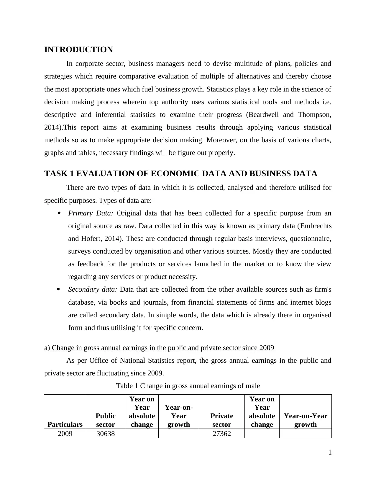
a) Change in gross annual earnings in the public and private sector since 2009
As per Office of National Statistics report, the gross annual earnings in the public and
private sector are fluctuating since 2009.
Table 1 Change in gross annual earnings of male
Particulars
Public
sector
Year on
Year
absolute
change
Year-on-
Year
growth
Private
sector
Year on
Year
absolute
change
Year-on-Year
growth
2009 30638 27362
1
In corporate sector, business managers need to devise multitude of plans, policies and
strategies which require comparative evaluation of multiple of alternatives and thereby choose
the most appropriate ones which fuel business growth. Statistics plays a key role in the science of
decision making process wherein top authority uses various statistical tools and methods i.e.
descriptive and inferential statistics to examine their progress (Beardwell and Thompson,
2014).This report aims at examining business results through applying various statistical
methods so as to make appropriate decision making. Moreover, on the basis of various charts,
graphs and tables, necessary findings will be figure out properly.
TASK 1 EVALUATION OF ECONOMIC DATA AND BUSINESS DATA
There are two types of data in which it is collected, analysed and therefore utilised for
specific purposes. Types of data are: Primary Data: Original data that has been collected for a specific purpose from an
original source as raw. Data collected in this way is known as primary data (Embrechts
and Hofert, 2014). These are conducted through regular basis interviews, questionnaire,
surveys conducted by organisation and other various sources. Mostly they are conducted
as feedback for the products or services launched in the market or to know the view
regarding any services or product necessity.
Secondary data: Data that are collected from the other available sources such as firm's
database, via books and journals, from financial statements of firms and internet blogs
are called secondary data. In simple words, the data which is already there in organised
form and thus utilising it for specific concern.
a) Change in gross annual earnings in the public and private sector since 2009
As per Office of National Statistics report, the gross annual earnings in the public and
private sector are fluctuating since 2009.
Table 1 Change in gross annual earnings of male
Particulars
Public
sector
Year on
Year
absolute
change
Year-on-
Year
growth
Private
sector
Year on
Year
absolute
change
Year-on-Year
growth
2009 30638 27362
1
2010 31264 626 2.04% 27000 -362 -1.32%
2011 31380 116 0.37% 27233 233 0.86%
2012 31816 436 1.39% 27705 472 1.73%
2013 32541 725 2.28% 28201 496 1.79%
2014 32878 337 1.04% 28442 241 0.85%
2015 33685 807 2.45% 28881 439 1.54%
2016 34011 326 0.97% 29679 798 2.76%
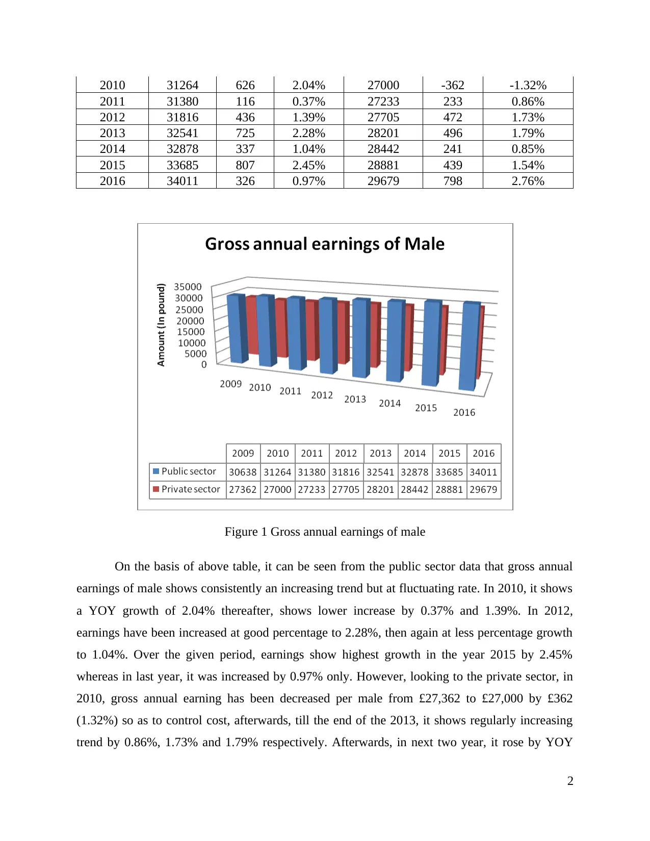
Figure 1 Gross annual earnings of male
On the basis of above table, it can be seen from the public sector data that gross annual
earnings of male shows consistently an increasing trend but at fluctuating rate. In 2010, it shows
a YOY growth of 2.04% thereafter, shows lower increase by 0.37% and 1.39%. In 2012,
earnings have been increased at good percentage to 2.28%, then again at less percentage growth
to 1.04%. Over the given period, earnings show highest growth in the year 2015 by 2.45%
whereas in last year, it was increased by 0.97% only. However, looking to the private sector, in
2010, gross annual earning has been decreased per male from £27,362 to £27,000 by £362
(1.32%) so as to control cost, afterwards, till the end of the 2013, it shows regularly increasing
trend by 0.86%, 1.73% and 1.79% respectively. Afterwards, in next two year, it rose by YOY
2
2011 31380 116 0.37% 27233 233 0.86%
2012 31816 436 1.39% 27705 472 1.73%
2013 32541 725 2.28% 28201 496 1.79%
2014 32878 337 1.04% 28442 241 0.85%
2015 33685 807 2.45% 28881 439 1.54%
2016 34011 326 0.97% 29679 798 2.76%
Figure 1 Gross annual earnings of male
On the basis of above table, it can be seen from the public sector data that gross annual
earnings of male shows consistently an increasing trend but at fluctuating rate. In 2010, it shows
a YOY growth of 2.04% thereafter, shows lower increase by 0.37% and 1.39%. In 2012,
earnings have been increased at good percentage to 2.28%, then again at less percentage growth
to 1.04%. Over the given period, earnings show highest growth in the year 2015 by 2.45%
whereas in last year, it was increased by 0.97% only. However, looking to the private sector, in
2010, gross annual earning has been decreased per male from £27,362 to £27,000 by £362
(1.32%) so as to control cost, afterwards, till the end of the 2013, it shows regularly increasing
trend by 0.86%, 1.73% and 1.79% respectively. Afterwards, in next two year, it rose by YOY
2
⊘ This is a preview!⊘
Do you want full access?
Subscribe today to unlock all pages.
Trusted by 1+ million students worldwide
growth of 0.85% and 1.54%. Recently, in 2016, it shows highest increase by 2.76% at a earning
of £29,679.
Table 2 Change in gross annual earnings of female
Particulars
Public
sector
Year on
Year
absolute
change
Year-on-
Year
growth
Private
sector
Year on
Year
absolute
change
Year-
on-
Year
growth
2009 25224 19551
2010 26113 889 3.52% 19532 -19 -0.10%
2011 26470 357 1.37% 19565 33 0.17%
2012 26636 166 0.63% 20313 748 3.82%
2013 27338 702 2.64% 20698 385 1.90%
2014 27705 367 1.34% 21017 319 1.54%
2015 27900 195 0.70% 21403 386 1.84%
2016 28053 153 0.55% 22251 848 3.96%
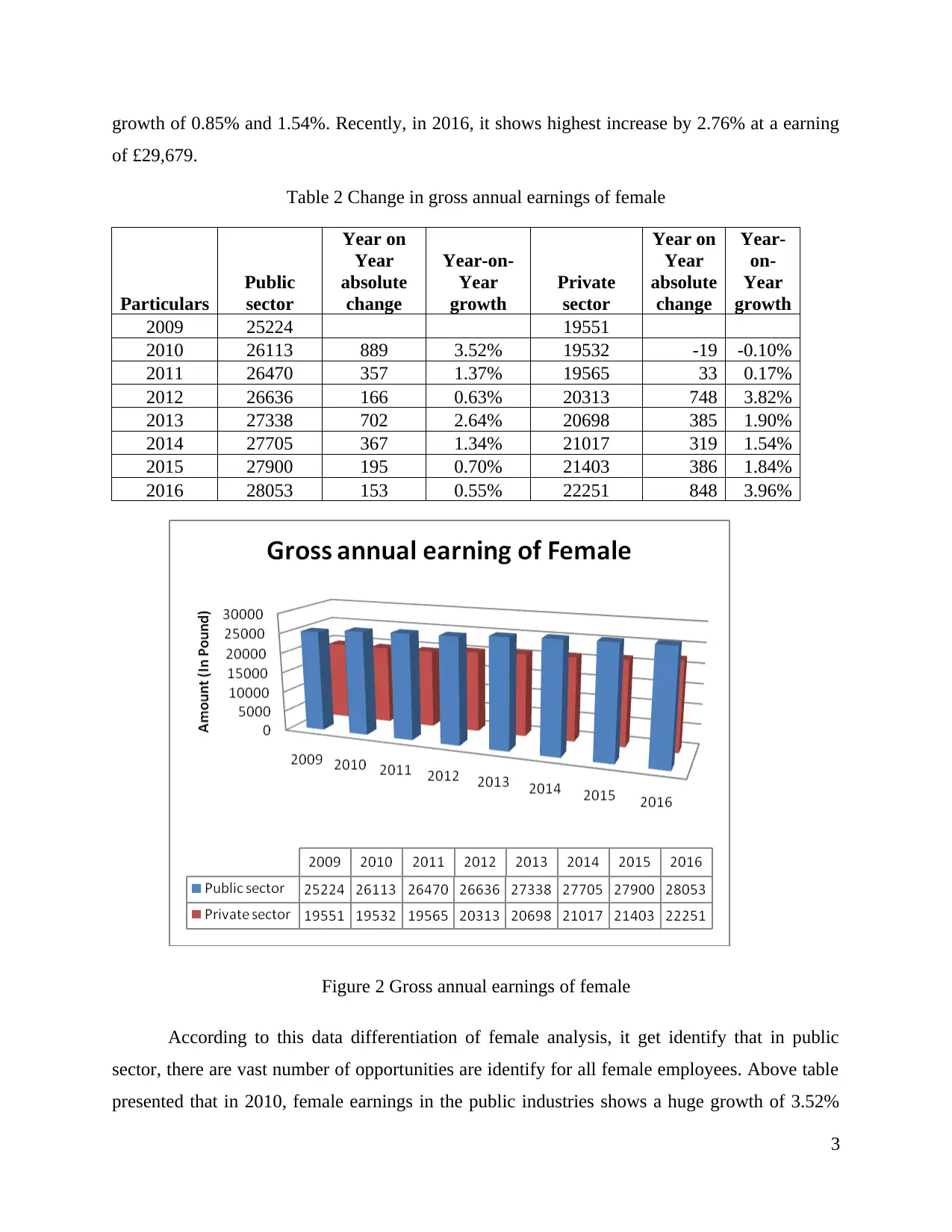
Figure 2 Gross annual earnings of female
According to this data differentiation of female analysis, it get identify that in public
sector, there are vast number of opportunities are identify for all female employees. Above table
presented that in 2010, female earnings in the public industries shows a huge growth of 3.52%
3
of £29,679.
Table 2 Change in gross annual earnings of female
Particulars
Public
sector
Year on
Year
absolute
change
Year-on-
Year
growth
Private
sector
Year on
Year
absolute
change
Year-
on-
Year
growth
2009 25224 19551
2010 26113 889 3.52% 19532 -19 -0.10%
2011 26470 357 1.37% 19565 33 0.17%
2012 26636 166 0.63% 20313 748 3.82%
2013 27338 702 2.64% 20698 385 1.90%
2014 27705 367 1.34% 21017 319 1.54%
2015 27900 195 0.70% 21403 386 1.84%
2016 28053 153 0.55% 22251 848 3.96%
Figure 2 Gross annual earnings of female
According to this data differentiation of female analysis, it get identify that in public
sector, there are vast number of opportunities are identify for all female employees. Above table
presented that in 2010, female earnings in the public industries shows a huge growth of 3.52%
3
Paraphrase This Document
Need a fresh take? Get an instant paraphrase of this document with our AI Paraphraser
whereas, in private sector, it came down by 0.10%. Afterwards, public sector shows an increase
but at declining rate by 1.37% and 0.63%, however, private sector shows an impressive growth
by 3.82% in 2012. Since 2014, although female workers in the public industries are paid with
higher wages, still, YOY growth is less by 1.34%, 0.70% and 0.55%. In contrast, private sector
workers were paid at high rate as their earning has been increased by 1.54%, 1.84% and 3.96%
respectively.
b) Gap between male and female annual earning
Table 3 Gap between male and female annual earnings in public sector
Public sector Male Female Gap
2009 30638 25224 5414
2010 31264 26113 5151
2011 31380 26470 4910
2012 31816 26636 5180
2013 32541 27338 5203
2014 32878 27705 5173
2015 33685 27900 5785
2016 34011 28053 5958
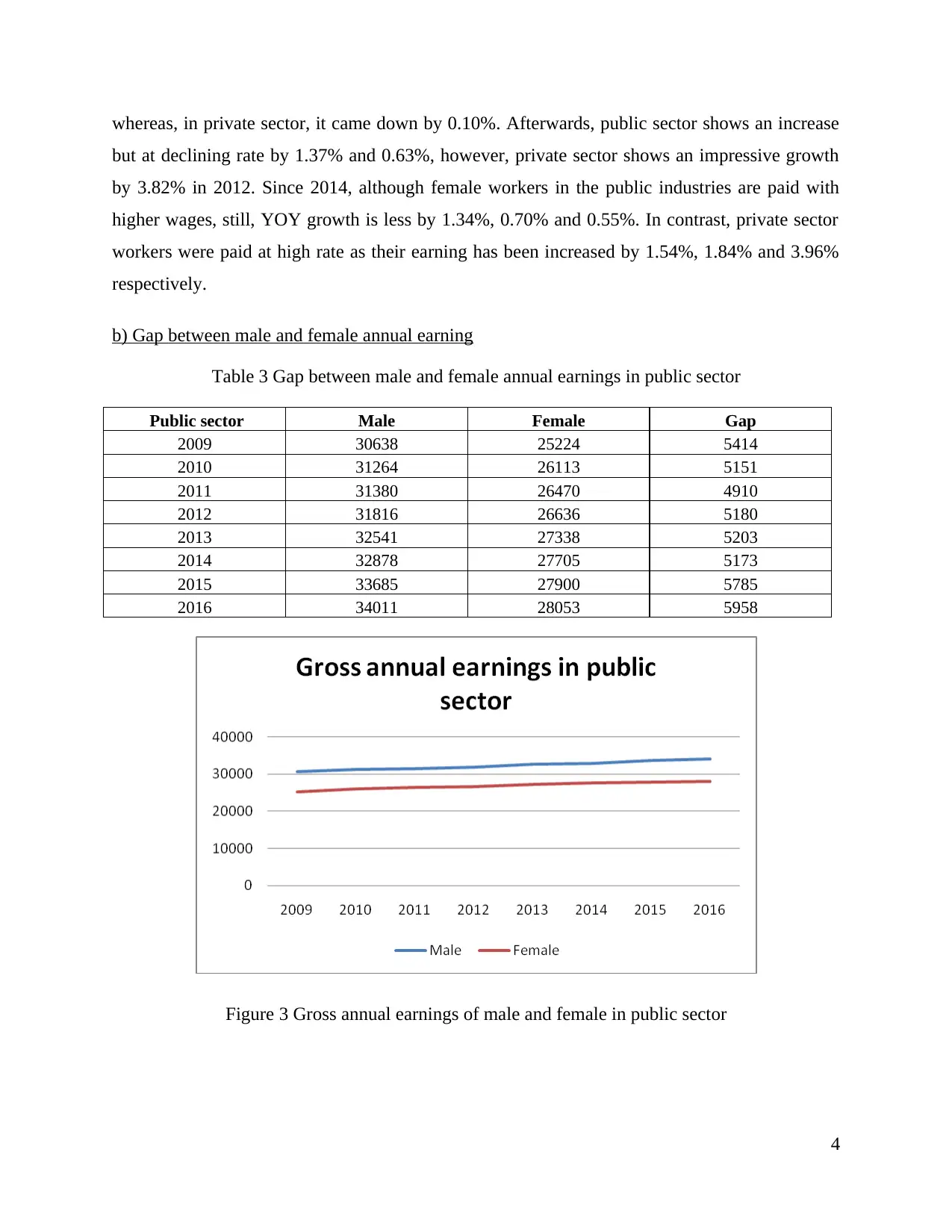
Figure 3 Gross annual earnings of male and female in public sector
4
but at declining rate by 1.37% and 0.63%, however, private sector shows an impressive growth
by 3.82% in 2012. Since 2014, although female workers in the public industries are paid with
higher wages, still, YOY growth is less by 1.34%, 0.70% and 0.55%. In contrast, private sector
workers were paid at high rate as their earning has been increased by 1.54%, 1.84% and 3.96%
respectively.
b) Gap between male and female annual earning
Table 3 Gap between male and female annual earnings in public sector
Public sector Male Female Gap
2009 30638 25224 5414
2010 31264 26113 5151
2011 31380 26470 4910
2012 31816 26636 5180
2013 32541 27338 5203
2014 32878 27705 5173
2015 33685 27900 5785
2016 34011 28053 5958
Figure 3 Gross annual earnings of male and female in public sector
4
As per the graph, male working in public sector always earn higher comparatively to
female workers. In 2016, the gap is highest by £5958 whereas year 2011 shows lowest gap by
£4910.
Table 4 Gap between male and female annual earnings in public sector
Private sector Male Female Gap
2009 27362 19551 7811
2010 27000 19532 7468
2011 27233 19565 7668
2012 27705 20313 7392
2013 28201 20698 7503
2014 28442 21017 7425
2015 28881 21403 7478
2016 29679 22251 7428
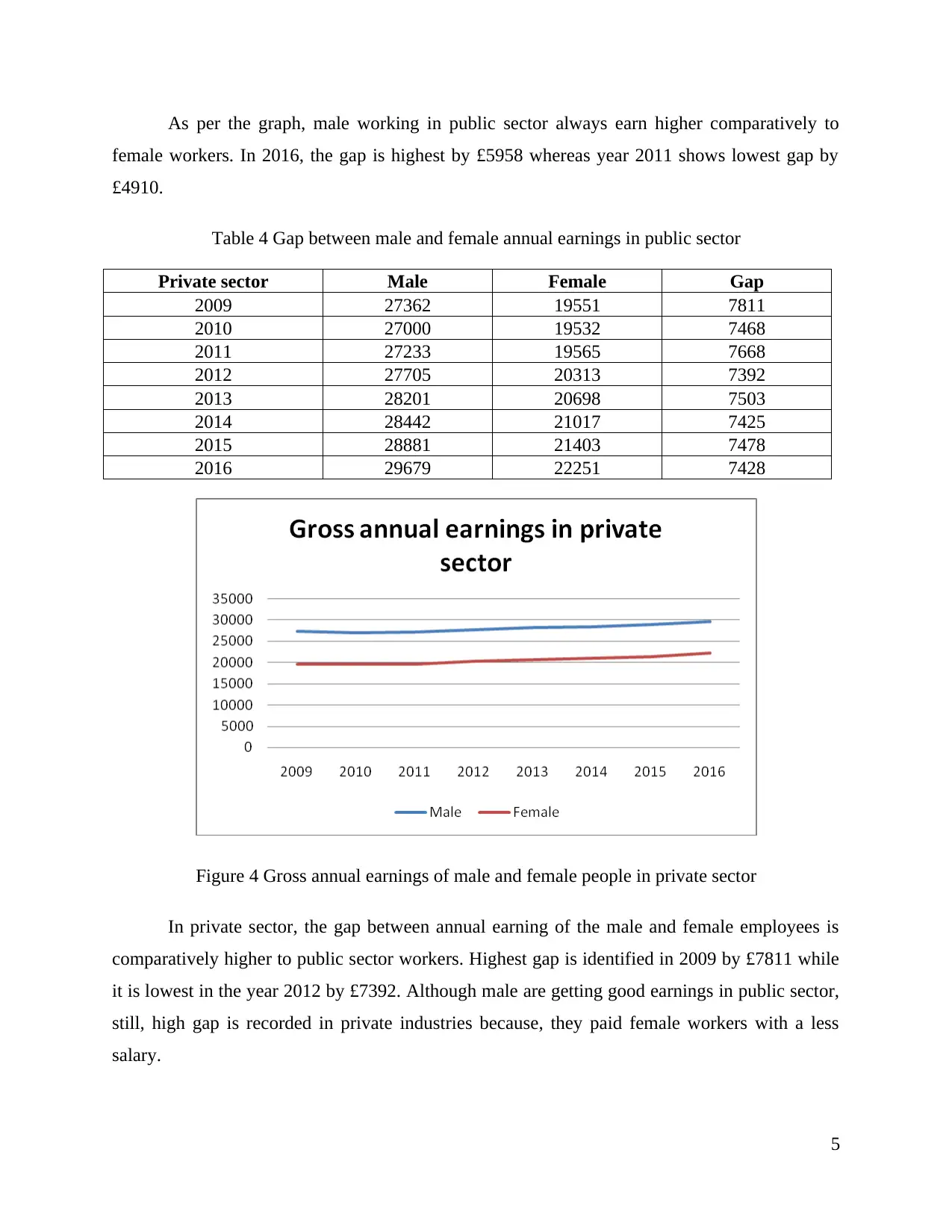
Figure 4 Gross annual earnings of male and female people in private sector
In private sector, the gap between annual earning of the male and female employees is
comparatively higher to public sector workers. Highest gap is identified in 2009 by £7811 while
it is lowest in the year 2012 by £7392. Although male are getting good earnings in public sector,
still, high gap is recorded in private industries because, they paid female workers with a less
salary.
5
female workers. In 2016, the gap is highest by £5958 whereas year 2011 shows lowest gap by
£4910.
Table 4 Gap between male and female annual earnings in public sector
Private sector Male Female Gap
2009 27362 19551 7811
2010 27000 19532 7468
2011 27233 19565 7668
2012 27705 20313 7392
2013 28201 20698 7503
2014 28442 21017 7425
2015 28881 21403 7478
2016 29679 22251 7428
Figure 4 Gross annual earnings of male and female people in private sector
In private sector, the gap between annual earning of the male and female employees is
comparatively higher to public sector workers. Highest gap is identified in 2009 by £7811 while
it is lowest in the year 2012 by £7392. Although male are getting good earnings in public sector,
still, high gap is recorded in private industries because, they paid female workers with a less
salary.
5
⊘ This is a preview!⊘
Do you want full access?
Subscribe today to unlock all pages.
Trusted by 1+ million students worldwide
TASK 2 ANALYSE AND EVALUATE RAW BUSINESS DATA USING
NUMBER OF STATISTICAL METHODS
Mainly there are two types of analysis which are used for every aspect of economic and
business aspect: Qualitative Analysis: There are certain aims and objectives which needs to be achieved
by using Interviews, Group discussion, experiments etc. In simple words it is a process in
which we move from the raw data that is being collected as part of research to provide
explanations, understanding and the process along with people in the research study. Aim
of analysing is to examine the meaningful content (Guan and Zhao, 2012).
Quantitative Analysis: It is an analysis that uses subjective judgement based on
unorganized information like management expertise, strength of research and
development and labour relations. It focuses on numbers that can be found on balance
sheet reports. Techniques will often be used in order to examine a organization's
operations and evaluate its potential as an investment opportunity.
A. (i) Use an Ogive to estimate the median hourly earnings
Median: Process of separating the higher half of data from the lower half or in simple
words the middle number (Keller, 2014).
Quartile: The quartiles of a ranked set of data values are three points that divide the data
set into for equal groups, each group comprising a quarter of data. The middle number between
the smallest number and median of data set is called the first quartile. Data's median is set as
second quartile and middle value between the median and the highest value of the data set is
known as third quartile.
Table 5 Calculation of cumulative frequency
Hourly earnings
(CI) F
Relative
frequency
Cumulative
frequency
Cumulative relative
frequency
0-10 8 8% 8 8%
10-20 46 46% 54 54%
20-30 26 26% 80 80%
30-40 14 14% 94 94%
40-50 6 6% 100 100%
10
0
6
Paraphrase This Document
Need a fresh take? Get an instant paraphrase of this document with our AI Paraphraser
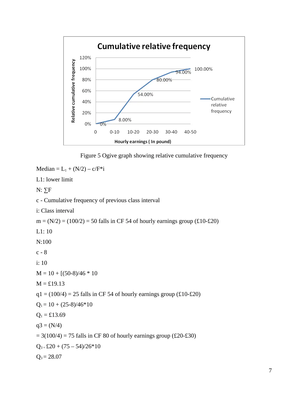
Figure 5 Ogive graph showing relative cumulative frequency
Median = L1 + (N/2) – c/F*i
L1: lower limit
N: ∑F
c - Cumulative frequency of previous class interval
i: Class interval
m = (N/2) = (100/2) = 50 falls in CF 54 of hourly earnings group (£10-£20)
L1: 10
N:100
c - 8
i: 10
M = 10 + [(50-8)/46 * 10
M = £19.13
q1 = (100/4) = 25 falls in CF 54 of hourly earnings group (£10-£20)
Q1 = 10 + (25-8)/46*10
Q1 = £13.69
q3 = (N/4)
= 3(100/4) = 75 falls in CF 80 of hourly earnings group (£20-£30)
Q3 = £20 + (75 – 54)/26*10
Q3 = 28.07
7
As per the results, median hourly earning of the workers is determined to £19.13 which is
near to wages rate £19/hour. It shows that 50% of the total employee base generates hourly
wages rate below £19 and rest of the employees are being paid at wages rate beyond £19 per
hour. As per the value of quartile, 25% of the workers are paid at wages rate below or equal to
£13.69 which is near to £14/hour and 75% have been paid at £28/hour. However, only 6
employees are paid at under the wages group of £40-£50.
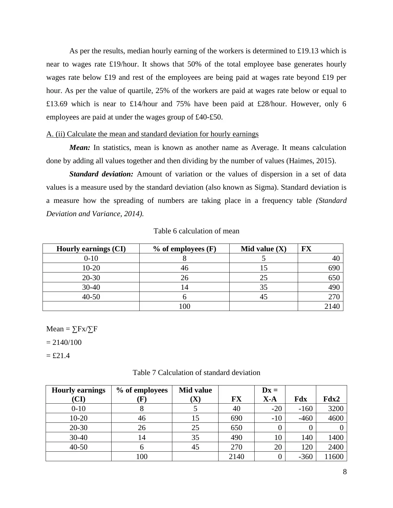
A. (ii) Calculate the mean and standard deviation for hourly earnings
Mean: In statistics, mean is known as another name as Average. It means calculation
done by adding all values together and then dividing by the number of values (Haimes, 2015).
Standard deviation: Amount of variation or the values of dispersion in a set of data
values is a measure used by the standard deviation (also known as Sigma). Standard deviation is
a measure how the spreading of numbers are taking place in a frequency table (Standard
Deviation and Variance, 2014).
Table 6 calculation of mean
Hourly earnings (CI) % of employees (F) Mid value (X) FX
0-10 8 5 40
10-20 46 15 690
20-30 26 25 650
30-40 14 35 490
40-50 6 45 270
100 2140
Mean = ∑Fx/∑F
= 2140/100
= £21.4
Table 7 Calculation of standard deviation
Hourly earnings
(CI)
% of employees
(F)
Mid value
(X) FX
Dx =
X-A Fdx Fdx2
0-10 8 5 40 -20 -160 3200
10-20 46 15 690 -10 -460 4600
20-30 26 25 650 0 0 0
30-40 14 35 490 10 140 1400
40-50 6 45 270 20 120 2400
100 2140 0 -360 11600
8
near to wages rate £19/hour. It shows that 50% of the total employee base generates hourly
wages rate below £19 and rest of the employees are being paid at wages rate beyond £19 per
hour. As per the value of quartile, 25% of the workers are paid at wages rate below or equal to
£13.69 which is near to £14/hour and 75% have been paid at £28/hour. However, only 6
employees are paid at under the wages group of £40-£50.
A. (ii) Calculate the mean and standard deviation for hourly earnings
Mean: In statistics, mean is known as another name as Average. It means calculation
done by adding all values together and then dividing by the number of values (Haimes, 2015).
Standard deviation: Amount of variation or the values of dispersion in a set of data
values is a measure used by the standard deviation (also known as Sigma). Standard deviation is
a measure how the spreading of numbers are taking place in a frequency table (Standard
Deviation and Variance, 2014).
Table 6 calculation of mean
Hourly earnings (CI) % of employees (F) Mid value (X) FX
0-10 8 5 40
10-20 46 15 690
20-30 26 25 650
30-40 14 35 490
40-50 6 45 270
100 2140
Mean = ∑Fx/∑F
= 2140/100
= £21.4
Table 7 Calculation of standard deviation
Hourly earnings
(CI)
% of employees
(F)
Mid value
(X) FX
Dx =
X-A Fdx Fdx2
0-10 8 5 40 -20 -160 3200
10-20 46 15 690 -10 -460 4600
20-30 26 25 650 0 0 0
30-40 14 35 490 10 140 1400
40-50 6 45 270 20 120 2400
100 2140 0 -360 11600
8
⊘ This is a preview!⊘
Do you want full access?
Subscribe today to unlock all pages.
Trusted by 1+ million students worldwide
1 out of 23
Related Documents


Your All-in-One AI-Powered Toolkit for Academic Success.
+13062052269
info@desklib.com
Available 24*7 on WhatsApp / Email
![[object Object]](/_next/static/media/star-bottom.7253800d.svg)
Unlock your academic potential
Copyright © 2020–2026 A2Z Services. All Rights Reserved. Developed and managed by ZUCOL.