ME5112 Math Assessment: Applying Mathematical Concepts and Methods
VerifiedAdded on 2023/04/21
|12
|2189
|244
Homework Assignment
AI Summary
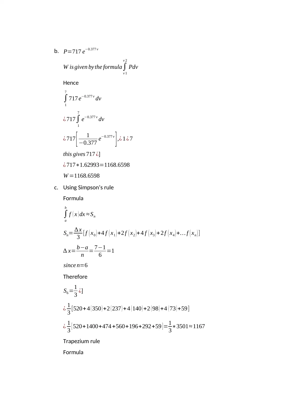
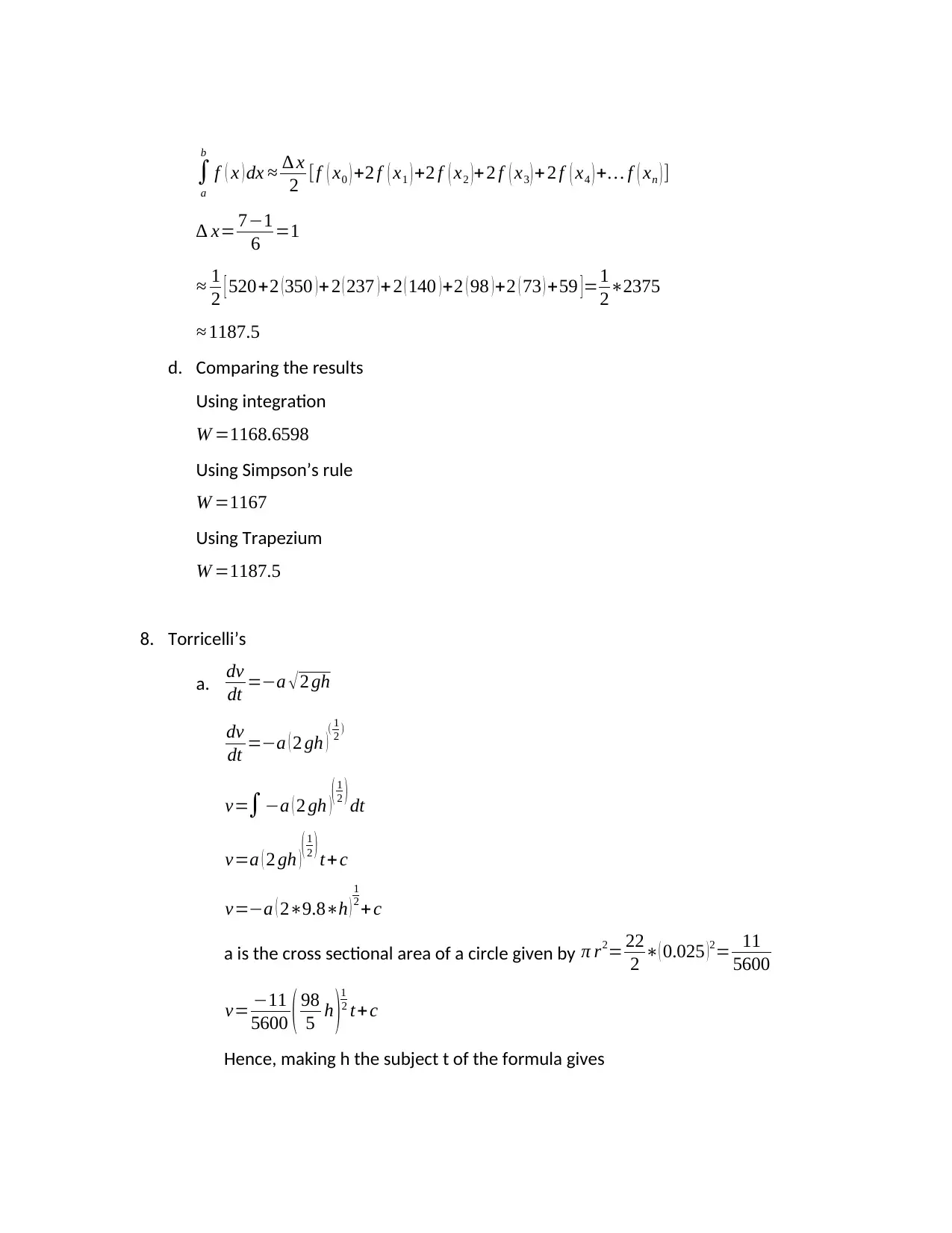
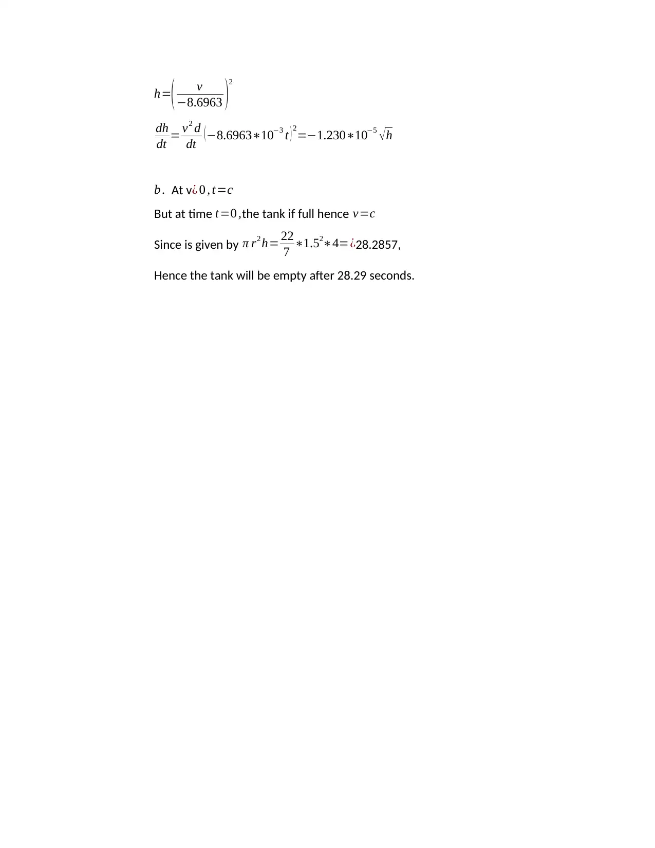
This document presents a comprehensive solution to a mathematics assessment, covering a range of topics including solving differential equations, applying Maclaurin and Taylor series for approximations, calculating eigenvalues and eigenvectors of a matrix, and using Euler's method to approximate solutions to differential equations related to Newton's law of cooling. The solution also includes graphical analysis of pressure and volume data, numerical integration using Simpson's and Trapezium rules, and an application of Torricelli's law to determine the emptying time of a tank. Each problem is addressed with detailed steps and explanations, providing a thorough understanding of the mathematical concepts and methods involved.
1 out of 12
Related Documents


Your All-in-One AI-Powered Toolkit for Academic Success.
+13062052269
info@desklib.com
Available 24*7 on WhatsApp / Email
![[object Object]](/_next/static/media/star-bottom.7253800d.svg)
Copyright © 2020–2025 A2Z Services. All Rights Reserved. Developed and managed by ZUCOL.