MECH419/928 : Simulation Assignment
VerifiedAdded on 2022/09/11
|19
|2833
|14
AI Summary
Contribute Materials
Your contribution can guide someone’s learning journey. Share your
documents today.
MECH419/928 1
Name
Institution
Name
Institution
Secure Best Marks with AI Grader
Need help grading? Try our AI Grader for instant feedback on your assignments.
MECH419/928 2
Simulation assignment
Part a
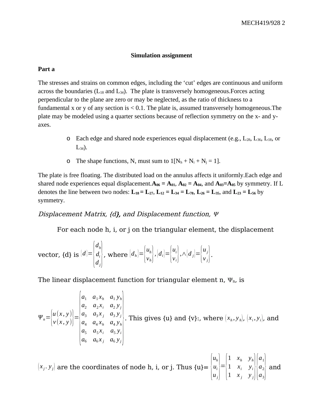
The stresses and strains on common edges, including the ‘cut’ edges are continuous and uniform
across the boundaries (L18 and L34). The plate is transversely homogeneous.Forces acting
perpendicular to the plane are zero or may be neglected, as the ratio of thickness to a
fundamental x or y of any section is < 0.1. The plate is, assumed transversely homogeneous.The
plate may be modeled using a quarter sections because of reflection symmetry on the x- and y-
axes.
o Each edge and shared node experiences equal displacement (e.g., L28, L36, L18, or
L34).
o The shape functions, N, must sum to 1[Nh + Ni + Nj = 1].
The plate is free floating. The distributed load on the annulus affects it uniformly.Each edge and
shared node experiences equal displacement.A06 = A01, A02 = A04, and A03=A05 by symmetry. If L
denotes the line between two nodes: L18 = L27, L12 = L34 = L78, L26 = L35, and L23 = L56 by
symmetry.
Displacement Matrix, {d}, and Displacement function,
For each node h, i, or j on the triangular element, the displacement
vector, {d} is { d }=
{dh
di
d j
}, where {dh }= {uh
vh }, {di }= {ui
vi },∧ {d j }= {u j
v j }.
The linear displacement function for triangular element n, n, is
Ψ n = {u (x , y )
v (x , y ) }=
{
a1
a2
a1 xh
a2 xi
a1 yh
a2 y j
a3 a3 x j a3 y j
a4
a5
a6
a4 xh
a5 xi
a6 x j
a4 yh
a5 yi
a6 y j
}. This gives {u} and {v}:, where ( xh , y h ), ( xi , yi ), and
( x j . y j ) are the coordinates of node h, i, or j. Thus {u}= {uh
ui
u j
}=
{1 xh yh
1 xi yi
1 x j y j
}{a1
a2
a3
} and
Simulation assignment
Part a
The stresses and strains on common edges, including the ‘cut’ edges are continuous and uniform
across the boundaries (L18 and L34). The plate is transversely homogeneous.Forces acting
perpendicular to the plane are zero or may be neglected, as the ratio of thickness to a
fundamental x or y of any section is < 0.1. The plate is, assumed transversely homogeneous.The
plate may be modeled using a quarter sections because of reflection symmetry on the x- and y-
axes.
o Each edge and shared node experiences equal displacement (e.g., L28, L36, L18, or
L34).
o The shape functions, N, must sum to 1[Nh + Ni + Nj = 1].
The plate is free floating. The distributed load on the annulus affects it uniformly.Each edge and
shared node experiences equal displacement.A06 = A01, A02 = A04, and A03=A05 by symmetry. If L
denotes the line between two nodes: L18 = L27, L12 = L34 = L78, L26 = L35, and L23 = L56 by
symmetry.
Displacement Matrix, {d}, and Displacement function,
For each node h, i, or j on the triangular element, the displacement
vector, {d} is { d }=
{dh
di
d j
}, where {dh }= {uh
vh }, {di }= {ui
vi },∧ {d j }= {u j
v j }.
The linear displacement function for triangular element n, n, is
Ψ n = {u (x , y )
v (x , y ) }=
{
a1
a2
a1 xh
a2 xi
a1 yh
a2 y j
a3 a3 x j a3 y j
a4
a5
a6
a4 xh
a5 xi
a6 x j
a4 yh
a5 yi
a6 y j
}. This gives {u} and {v}:, where ( xh , y h ), ( xi , yi ), and
( x j . y j ) are the coordinates of node h, i, or j. Thus {u}= {uh
ui
u j
}=
{1 xh yh
1 xi yi
1 x j y j
}{a1
a2
a3
} and
MECH419/928 3
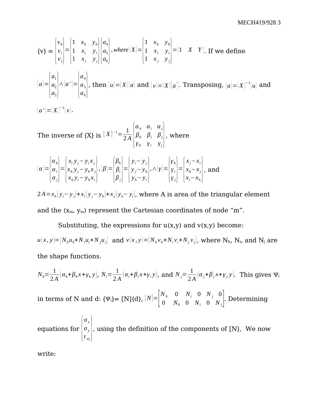
{v} = {
vh
vi
v j
}=
{
1 xh yh
1 xi yi
1 x j y j
}{
a4
a5
a6
} , where { Χ } =
{
1 xh yh
1 xi yi
1 x j y j
}= {1 X Y }. If we define
{ a }=
{a1
a2
a3
}∧ {a ' }=
{a4
a5
a6
}, then { u } = { X } { a } and { v }= { X } { a' }. Transposing, { a }= { Χ }−1 { u } and
{ a ' }= { Χ }−1 { v }.
The inverse of {X} is { Χ }−1= 1
2 A {α h α i α j
βh βi β j
γ h γi γj
}, where
{ α }=
{αh
α i
α j
}=
{ xi y j − yi x j
xh y j − yh x j
xh yi − yh xi
}, { β }=
{βh
βi
β j
}=
{ yi− y j
y j− yh
yh− yi
},∧ { γ }=
{γ h
γ i
γ j
}=
{ x j−xi
xh−x j
xi−xh
}, and
2 A=xh ( yi− y j ) + xi ( y j− yh ) + x j ( yh− yi ), where A is area of the triangular element
and the (xm, ym) represent the Cartesian coordinates of node “m”.
Substituting, the expressions for u(x,y) and v(x,y) become:
u ( x , y ) = { Nh uh+ N i ui + N j u j } and v ( x , y ) = { Nh vh +Ni vi +N j v j }, where Nh, Ni, and Nj are
the shape functions.
Nh= 1
2 A ( αh + βh x + γh y ), Ni= 1
2 A ( αi + βi x +γ i y ), and N j= 1
2 A ( α j +β j x+ γ j y ). This gives i
in terms of N and d: {i}= [N]{d}, [ N ] = [ N h 0 Ni 0 N j 0
0 Nh 0 Ni 0 N j ]. Determining
equations for {σ x
σ y
τ xy
}, using the definition of the components of [N}, We now
write:
MECH419/928 4
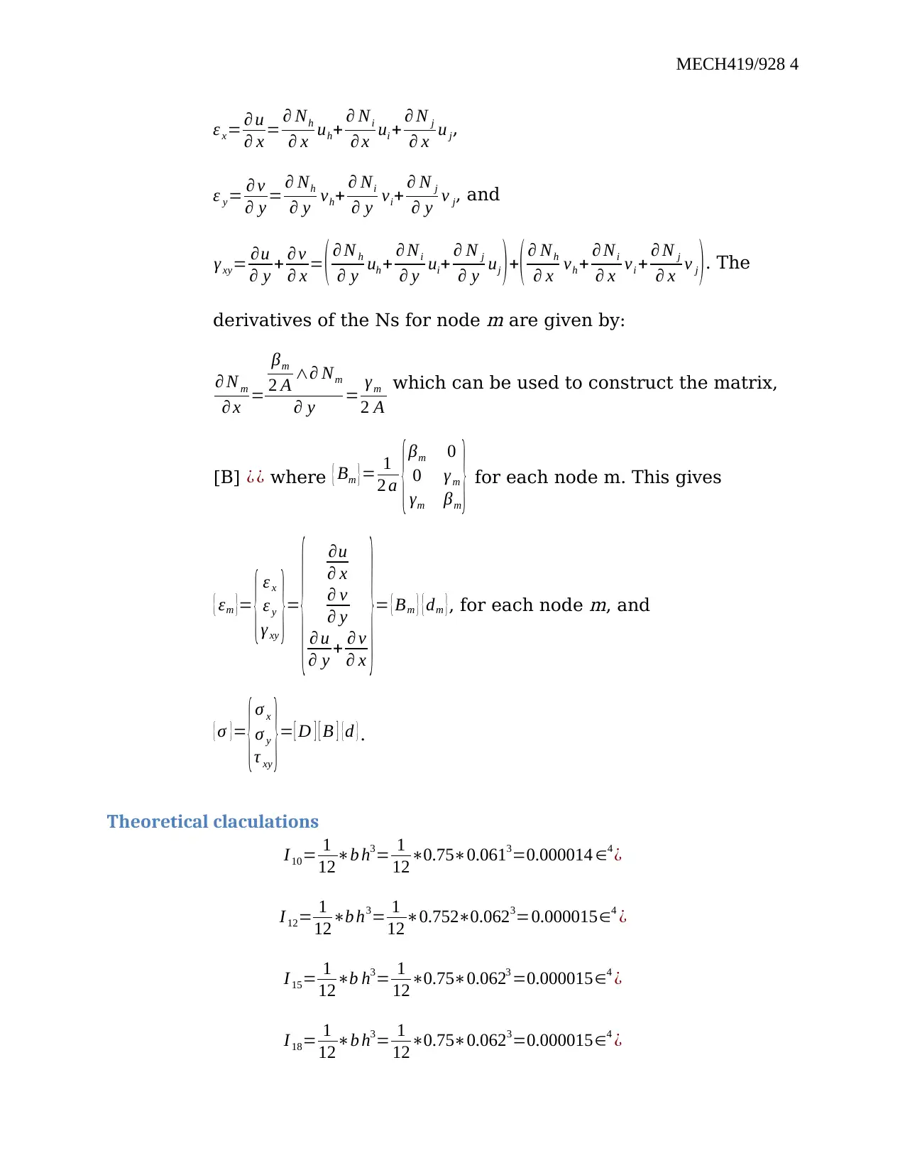
ε x= ∂ u
∂ x = ∂ Nh
∂ x uh+ ∂ Ni
∂ x ui + ∂ N j
∂ x u j,
ε y= ∂ v
∂ y = ∂ Nh
∂ y vh+ ∂ Ni
∂ y vi+ ∂ N j
∂ y v j, and
γ xy= ∂u
∂ y + ∂ v
∂ x = ( ∂ N h
∂ y uh + ∂ Ni
∂ y ui+ ∂ N j
∂ y uj )+( ∂ Nh
∂ x vh + ∂ Ni
∂ x vi + ∂ N j
∂ x v j ). The
derivatives of the Ns for node
m are given by:
∂ N m
∂ x =
βm
2 A ∧∂ Nm
∂ y = γm
2 A
which can be used to construct the matrix,
[B] ¿ ¿ where { Bm }= 1
2 a {βm 0
0 γ m
γm βm
} for each node m. This gives
{ εm }= { ε x
ε y
γ xy
}=
{ ∂u
∂ x
∂ v
∂ y
∂ u
∂ y + ∂ v
∂ x
}= { Bm } { dm }, for each node
m, and
{ σ }=
{σ x
σ y
τ xy
}= [ D ] [ B ] {d }.
Theoretical claculations
I10= 1
12∗b h3= 1
12∗0.75∗0.0613=0.000014 ∈4 ¿
I 12= 1
12∗b h3= 1
12∗0.752∗0.0623=0.000015∈4 ¿
I 15= 1
12∗b h3= 1
12∗0.75∗0.0623 =0.000015∈4 ¿
I 18= 1
12∗b h3= 1
12∗0.75∗0.0623=0.000015∈4 ¿
Secure Best Marks with AI Grader
Need help grading? Try our AI Grader for instant feedback on your assignments.
MECH419/928 5
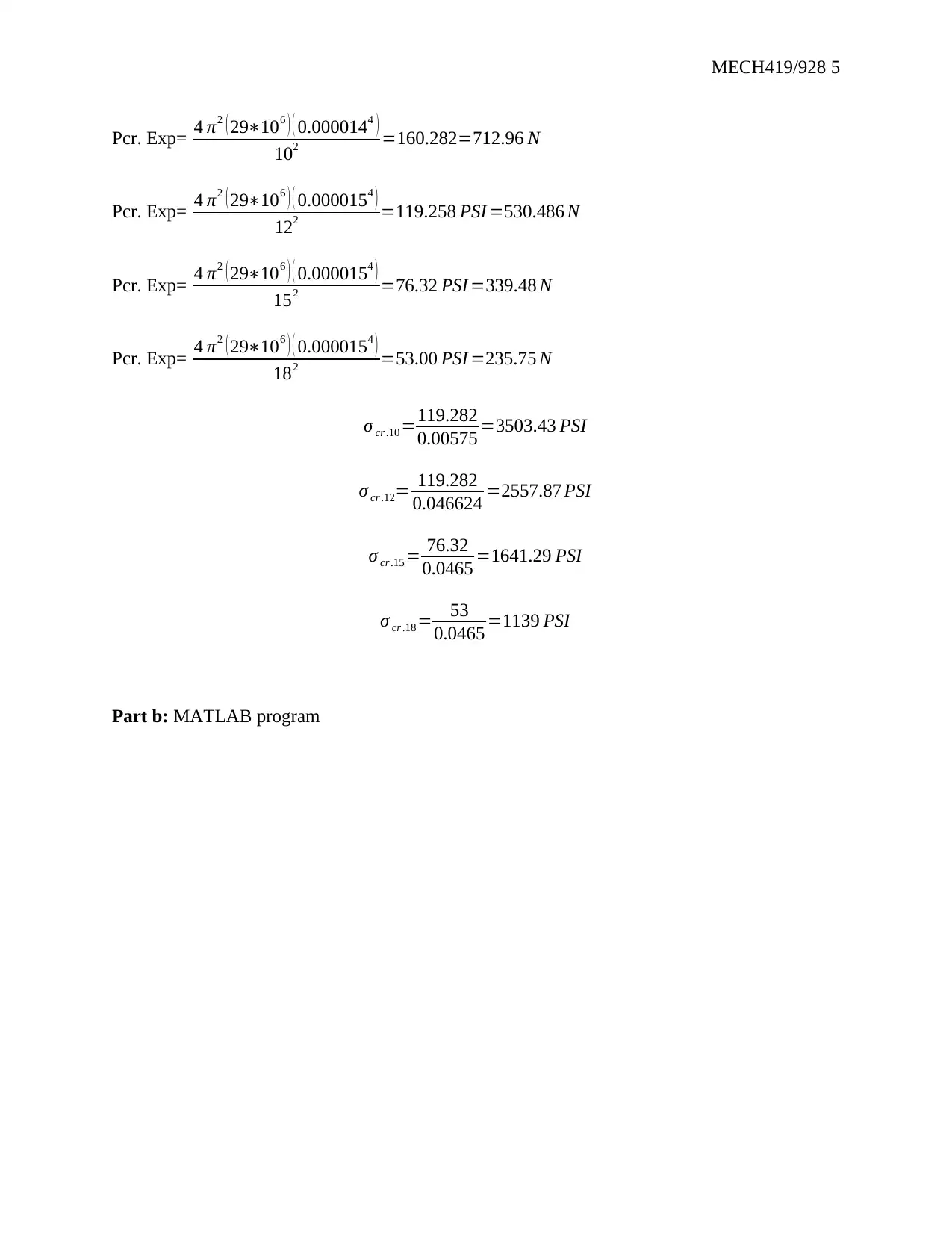
Pcr. Exp= 4 π2 ( 29∗106 ) ( 0.0000144 )
102 =160.282=712.96 N
Pcr. Exp= 4 π2 ( 29∗106 ) ( 0.0000154 )
122 =119.258 PSI =530.486 N
Pcr. Exp= 4 π2 ( 29∗106 ) ( 0.0000154 )
152 =76.32 PSI =339.48 N
Pcr. Exp= 4 π2 ( 29∗106 ) ( 0.0000154 )
182 =53.00 PSI =235.75 N
σ cr .10=119.282
0.00575 =3503.43 PSI
σ cr .12= 119.282
0.046624 =2557.87 PSI
σ cr.15 = 76.32
0.0465 =1641.29 PSI
σ cr .18= 53
0.0465 =1139 PSI
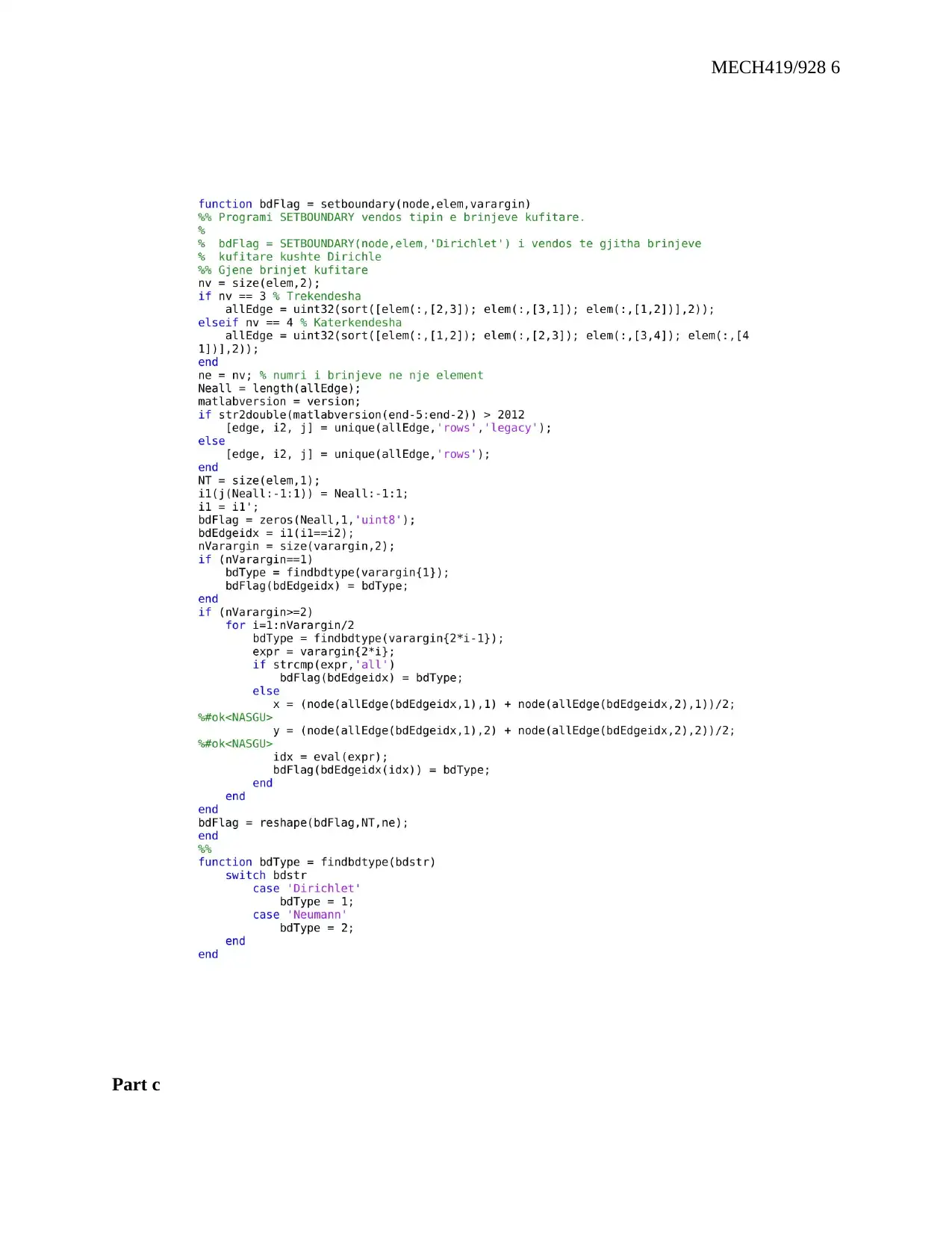
Part b: MATLAB program
Pcr. Exp= 4 π2 ( 29∗106 ) ( 0.0000144 )
102 =160.282=712.96 N
Pcr. Exp= 4 π2 ( 29∗106 ) ( 0.0000154 )
122 =119.258 PSI =530.486 N
Pcr. Exp= 4 π2 ( 29∗106 ) ( 0.0000154 )
152 =76.32 PSI =339.48 N
Pcr. Exp= 4 π2 ( 29∗106 ) ( 0.0000154 )
182 =53.00 PSI =235.75 N
σ cr .10=119.282
0.00575 =3503.43 PSI
σ cr .12= 119.282
0.046624 =2557.87 PSI
σ cr.15 = 76.32
0.0465 =1641.29 PSI
σ cr .18= 53
0.0465 =1139 PSI
Part b: MATLAB program
MECH419/928 6
Part c
Part c
MECH419/928 7
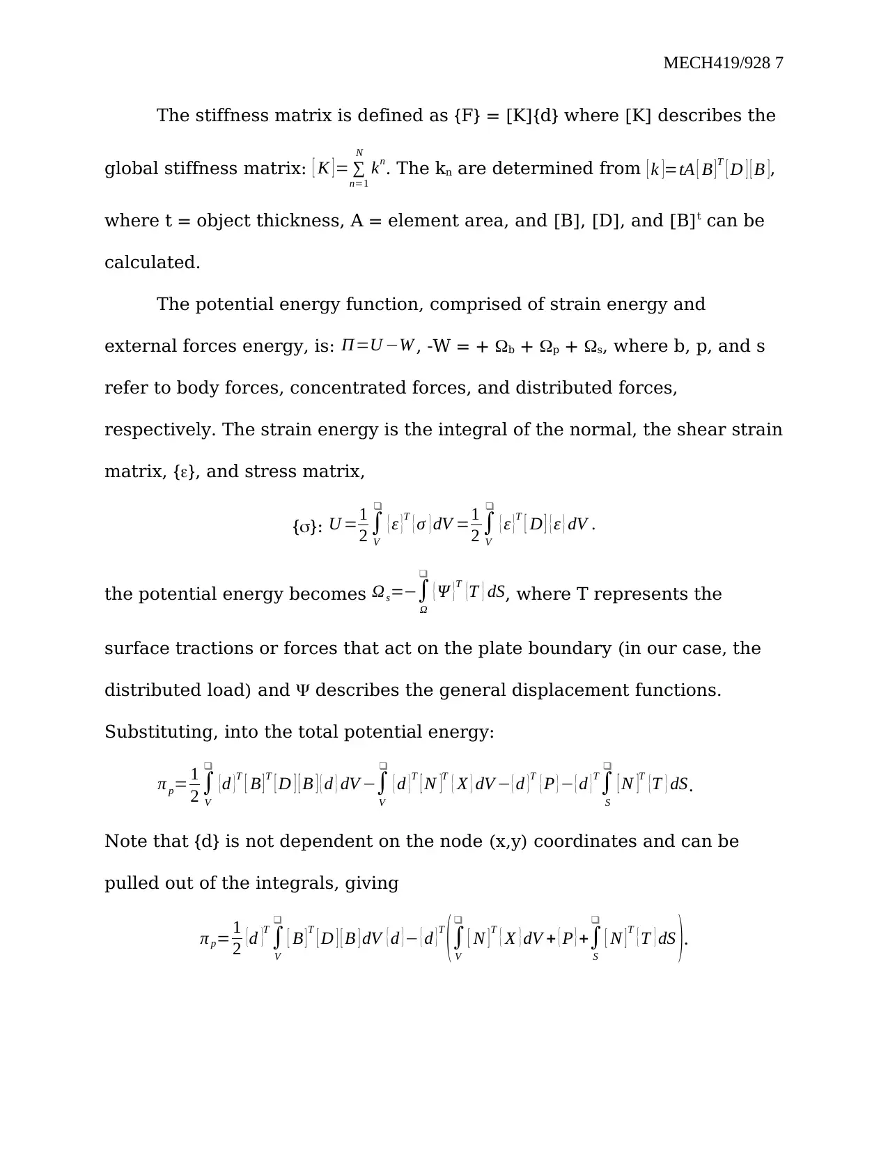
The stiffness matrix is defined as {F} = [K]{d} where [K] describes the
global stiffness matrix: [ K ] = ∑
n=1
N
kn. The kn are determined from [ k ]=tA [ B ] T [ D ] [ B ],
where t = object thickness, A = element area, and [B], [D], and [B]t can be
calculated.
The potential energy function, comprised of strain energy and
external forces energy, is: Π=U −W , -W = + b + p + s, where b, p, and s
refer to body forces, concentrated forces, and distributed forces,
respectively. The strain energy is the integral of the normal, the shear strain
matrix, {}, and stress matrix,
{}: U =1
2 ∫
V
❑
{ ε }
T { σ } dV =1
2 ∫
V
❑
{ ε }
T [ D ] { ε } dV .
the potential energy becomes Ωs=−∫
Ω
❑
{ Ψ }T {T } dS, where T represents the
surface tractions or forces that act on the plate boundary (in our case, the
distributed load) and describes the general displacement functions.
Substituting, into the total potential energy:
π p= 1
2 ∫
V
❑
{d }T [ B ] T [ D ] [ B ] { d } dV −∫
V
❑
{ d }T [ N ]T { X } dV − { d }T { P } − { d }T
∫
S
❑
[ N ]T {T } dS.
Note that {d} is not dependent on the node (x,y) coordinates and can be
pulled out of the integrals, giving
π p= 1
2 {d }T
∫
V
❑
[ B ] T
[ D ] [ B ] dV { d }− { d }T
(∫
V
❑
[ N ] T { X } dV + { P } +∫
S
❑
[ N ] T { T } dS ).
Paraphrase This Document
Need a fresh take? Get an instant paraphrase of this document with our AI Paraphraser

MECH419/928 8
The last three terms in the previous expression define the nodal force
vector, f,.
{ f }=∫
V
❑
[ N ]T { X } dV ± { P }+∫
S
❑
[ N ]T { T } dS.
Writing potential energy as π p= 1
2 {d }T
(∫
V
❑
[ B ]T
[ D ] [ B ] dV ) { d }− { d }T
{f }, it can be
minimized to determine the force vector ( ∂ π p
∂ { d } =0 ¿. The expression for { f } is
{ f }=∫
V
❑
[ B ] t [ D ] [ B ] dV { d }, where the stiffness matrix, k, is defined: [ k ]=∫
V
❑
[ B ] t [ D ] [ B ] dV
.
For a body with constant thickness, t can be pulled out as a constant.
The integral over the volume, V, becomes the integral over area, A, and the
expression for [k] becomes [ k ]=t∫
A
❑
[ B ]t [ D ] [ B ] dXdY . The two dimensional
integral has no x or y dependence except dXdY, so the integral just adds
area term to the integrand. The new expression becomes [ k ]=t [ B ]t [ D ] [ B ] A,
where A is the element area.
The [k] matrix for all three nodes is:
[ k ]=
[ [ khh ] [ khi ] [ khj ]
[ kih ] [ kii ] [ kij ]
[ k jh ] [ k ji ] [ k jj ] ], where the expression for any element in the matrix
follows this convention for solution: [ k hi ] =t [ Bh ] t [ D ] [ Bi ] A.
MECH419/928 9
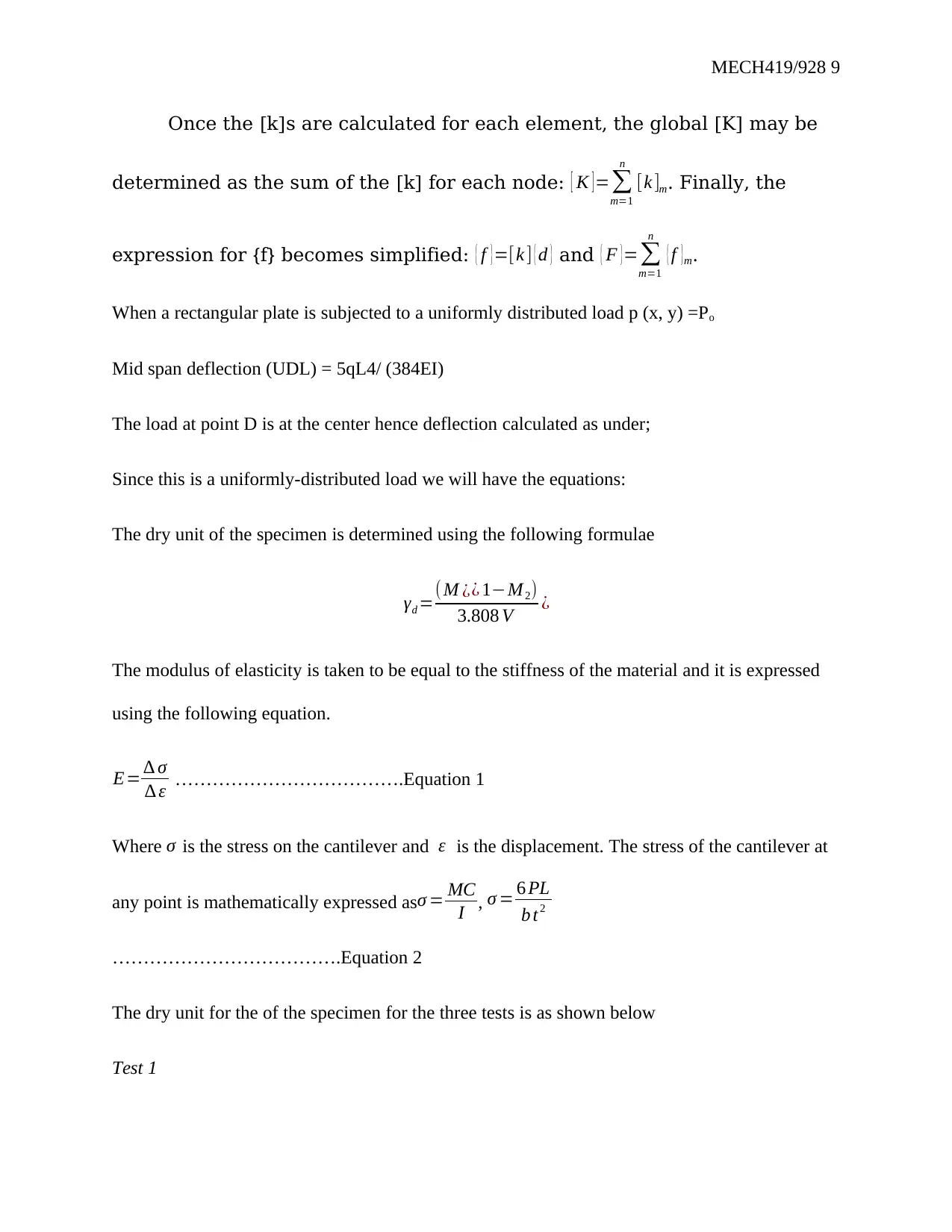
Once the [k]s are calculated for each element, the global [K] may be
determined as the sum of the [k] for each node: [ K ] =∑
m=1
n
[k ]m. Finally, the
expression for {f} becomes simplified: { f }=[k ] { d } and { F }=∑
m=1
n
{ f }m.
When a rectangular plate is subjected to a uniformly distributed load p (x, y) =Po
Mid span deflection (UDL) = 5qL4/ (384EI)
The load at point D is at the center hence deflection calculated as under;
Since this is a uniformly-distributed load we will have the equations:
The dry unit of the specimen is determined using the following formulae
γd =( M ¿¿ 1−M2)
3.808 V ¿
The modulus of elasticity is taken to be equal to the stiffness of the material and it is expressed
using the following equation.
E= ∆ σ
∆ ε ……………………………….Equation 1
Where σ is the stress on the cantilever and ε is the displacement. The stress of the cantilever at
any point is mathematically expressed asσ = MC
I , σ = 6 PL
b t2
……………………………….Equation 2
The dry unit for the of the specimen for the three tests is as shown below
Test 1
MECH419/928 10
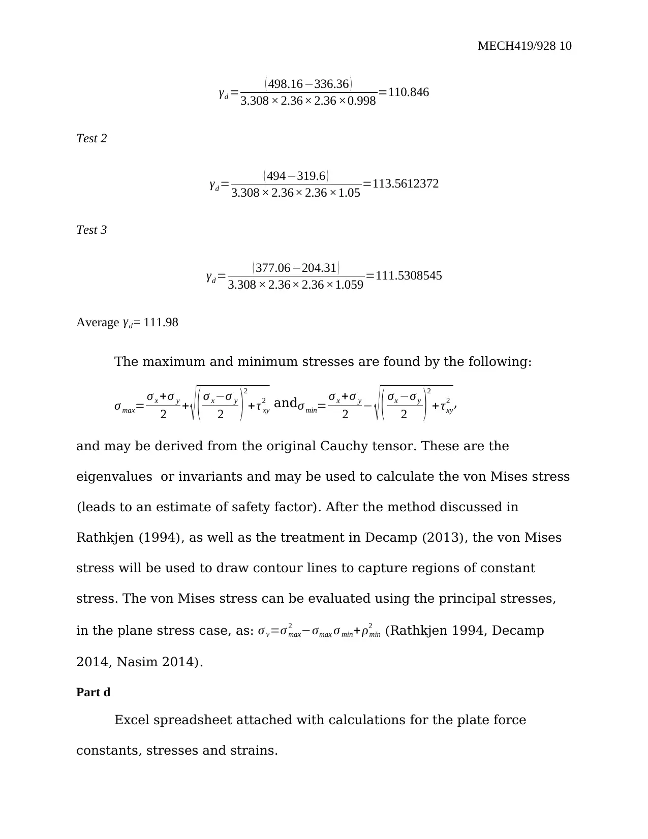
γd = ( 498.16−336.36 )
3.308 × 2.36× 2.36 ×0.998 =110.846
Test 2
γd = ( 494−319.6 )
3.308 × 2.36× 2.36 ×1.05 =113.5612372
Test 3
γd = ( 377.06−204.31 )
3.308 × 2.36× 2.36 ×1.059 =111.5308545
Average γd= 111.98
The maximum and minimum stresses are found by the following:
σ max= σ x +σ y
2 + √ ( σ x−σ y
2 )2
+τ xy
2 andσ min= σ x +σ y
2 − √ ( σx −σ y
2 )2
+ τxy
2 ,
and may be derived from the original Cauchy tensor. These are the
eigenvalues or invariants and may be used to calculate the von Mises stress
(leads to an estimate of safety factor). After the method discussed in
Rathkjen (1994), as well as the treatment in Decamp (2013), the von Mises
stress will be used to draw contour lines to capture regions of constant
stress. The von Mises stress can be evaluated using the principal stresses,
in the plane stress case, as: σ v=σ max
2 −σmax σ min+ ρmin
2 (Rathkjen 1994, Decamp
2014, Nasim 2014).
Part d
Excel spreadsheet attached with calculations for the plate force
constants, stresses and strains.
Secure Best Marks with AI Grader
Need help grading? Try our AI Grader for instant feedback on your assignments.
MECH419/928 11
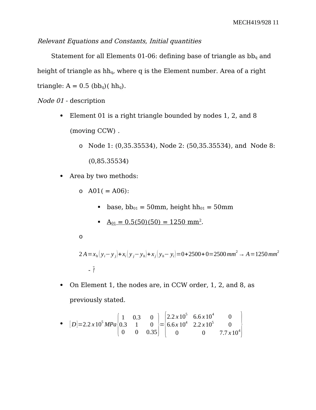
Relevant Equations and Constants, Initial quantities
Statement for all Elements 01-06: defining base of triangle as bbq and
height of triangle as hhq, where q is the Element number. Area of a right
triangle: A = 0.5 (bbq)( hhq).
Node 01 - description
Element 01 is a right triangle bounded by nodes 1, 2, and 8
(moving CCW) .
o Node 1: (0,35.35534), Node 2: (50,35.35534), and Node 8:
(0,85.35534)
Area by two methods:
o A01( = A06):
base, bb01 = 50mm, height hh01 = 50mm
A01 = 0.5(50)(50) = 1250 mm2.
o
2 A=xh ( yi− y j ) +xi ( y j− yh ) + x j ( yh− yi ) =0+2500+ 0=2500 mm2 → A=1250 mm2
- ˇ!
On Element 1, the nodes are, in CCW order, 1, 2, and 8, as
previously stated.
[ D ] =2.2 x 10⁵ MPa { 1 0.3 0
0.3 1 0
0 0 0.35 }= {2.2 x 10⁵ 6.6 x 10⁴ 0
6.6 x 10⁴ 2.2 x 10⁵ 0
0 0 7.7 x 10⁴ }
MECH419/928 12
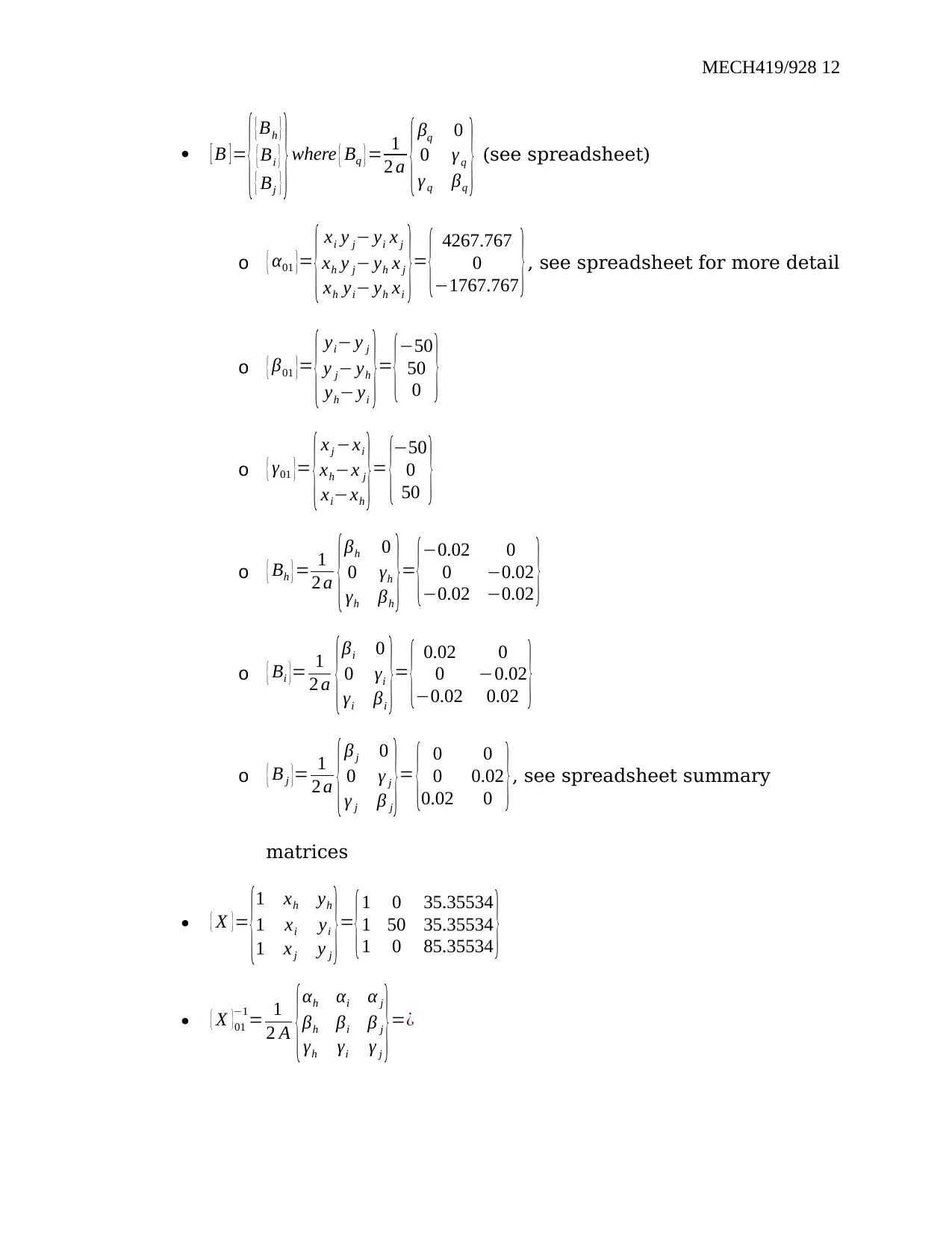
[ B ] =
{
{ Bh }
{ Bi }
{ Bj } } where { Bq } = 1
2 a { βq 0
0 γ q
γ q βq
} (see spreadsheet)
o { α01 }=
{ xi y j− yi x j
xh y j− yh x j
xh yi− yh xi
}= { 4267.767
0
−1767.767 }, see spreadsheet for more detail
o { β01 }=
{ yi− y j
y j− yh
yh− yi
}= {−50
50
0 }
o { γ01 }=
{x j −xi
xh−x j
xi−xh
}= {−50
0
50 }
o { Bh }= 1
2 a {βh 0
0 γh
γh βh
}= {−0.02 0
0 −0.02
−0.02 −0.02 }
o { Bi }= 1
2 a {βi 0
0 γi
γi βi
}= { 0.02 0
0 −0.02
−0.02 0.02 }
o { B j }= 1
2 a { β j 0
0 γ j
γ j β j
}= { 0 0
0 0.02
0.02 0 }, see spreadsheet summary
matrices
{ Χ }=
{1 xh yh
1 xi yi
1 x j y j
}= {1 0 35.35534
1 50 35.35534
1 0 85.35534 }
{ X }01
−1= 1
2 A {αh αi α j
βh βi β j
γh γi γ j
}=¿
MECH419/928 13
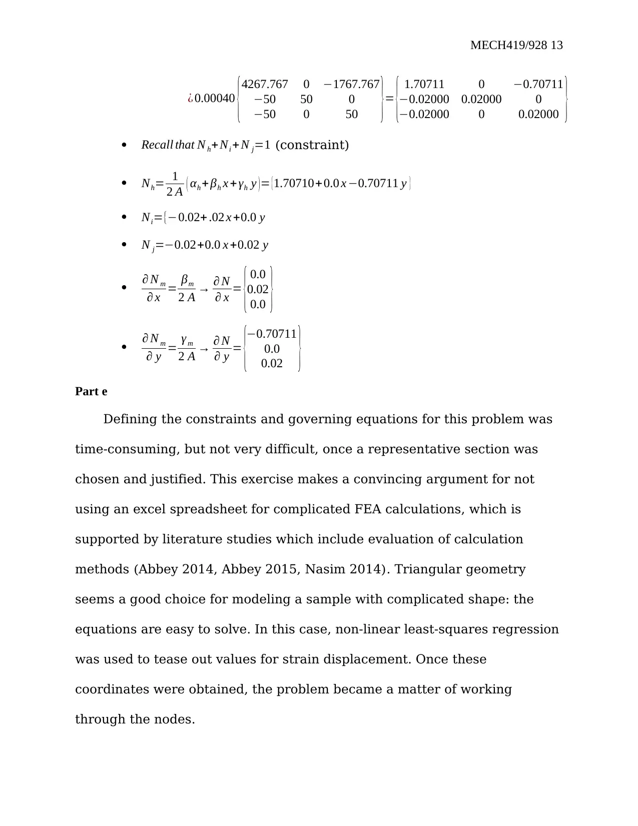
¿ 0.00040 {
4267.767 0 −1767.767
−50 50 0
−50 0 50 }= { 1.70711 0 −0.70711
−0.02000 0.02000 0
−0.02000 0 0.02000 }
Recall that N h+Ni + N j=1 (constraint)
Nh= 1
2 A ( αh + βh x + γh y )= {1.70710+ 0.0 x −0.70711 y }
Ni={−0.02+ .02 x +0.0 y
N j=−0.02+0.0 x +0.02 y
∂ N m
∂ x = βm
2 A → ∂ N
∂ x = { 0.0
0.02
0.0 }
∂ N m
∂ y = γ m
2 A → ∂ N
∂ y = {−0.70711
0.0
0.02 }
Part e
Defining the constraints and governing equations for this problem was
time-consuming, but not very difficult, once a representative section was
chosen and justified. This exercise makes a convincing argument for not
using an excel spreadsheet for complicated FEA calculations, which is
supported by literature studies which include evaluation of calculation
methods (Abbey 2014, Abbey 2015, Nasim 2014). Triangular geometry
seems a good choice for modeling a sample with complicated shape: the
equations are easy to solve. In this case, non-linear least-squares regression
was used to tease out values for strain displacement. Once these
coordinates were obtained, the problem became a matter of working
through the nodes.
Paraphrase This Document
Need a fresh take? Get an instant paraphrase of this document with our AI Paraphraser
MECH419/928 14
The condition that the plate is transversely homogeneous allowed
treatment in two dimensions. All hand-calculable quantites are included in
the excel sheet, and problem is ready for ANSYS analysis.Finite Element
Analysis is used to find the stresses, strains, stiffness matrix, and directional
vectors for any displacement experienced by this plate. It permits the
engineer to develop approximate solutions to a wide variety of problems
where understanding of force transfer, failure modes, stresses and strain, or
critical loads must be found where direct solution or measurement is
difficult, or where there are more variables and equations available than
knowns to describe the system. FEA originated in the aerospace industry to
model aircraft members or air flow and resistances in/on wings and other
surfaces, or explore flow features above and beneath an a air foil, dam, or
wing. Mallikarjun, et al. performed a series of calculations developing
methods and probing sensitivity of FEA in modeling flat, thin plates with
holes, similar to the project in this study (2012). Some of their methodology
been used for guidance. As well, model equations and assumptions are
outlined below. The goal is to develop the 2 dimensional general expression
and use constraints to build the approximations to solve for the stiffness
matrix.
The modulus of elasticity is given as the ratio of stress and strain of a material. Modulus of
elasticity gives the mechanical stiffness of the material and the deformation characteristics of the
MECH419/928 15
metal. Tensile strength is respect to the axial load applied and the nature of the load. Modulus
of elasticity is also known as Young’s Modulus.
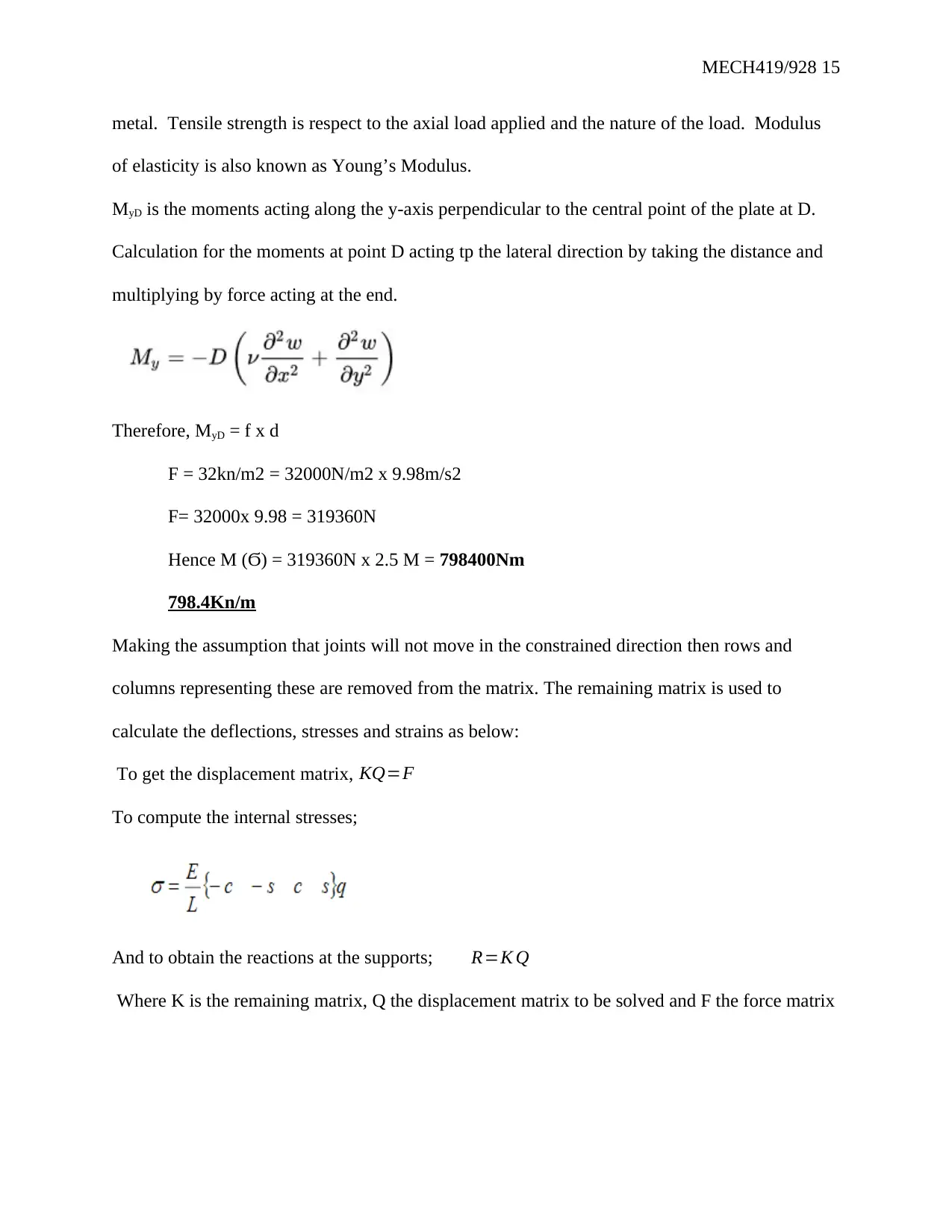
MyD is the moments acting along the y-axis perpendicular to the central point of the plate at D.
Calculation for the moments at point D acting tp the lateral direction by taking the distance and
multiplying by force acting at the end.
Therefore, MyD = f x d
F = 32kn/m2 = 32000N/m2 x 9.98m/s2
F= 32000x 9.98 = 319360N
Hence M (Ϭ) = 319360N x 2.5 M = 798400Nm
798.4Kn/m
Making the assumption that joints will not move in the constrained direction then rows and
columns representing these are removed from the matrix. The remaining matrix is used to
calculate the deflections, stresses and strains as below:
To get the displacement matrix, KQ=F
To compute the internal stresses;
And to obtain the reactions at the supports; R=K Q
Where K is the remaining matrix, Q the displacement matrix to be solved and F the force matrix
metal. Tensile strength is respect to the axial load applied and the nature of the load. Modulus
of elasticity is also known as Young’s Modulus.
MyD is the moments acting along the y-axis perpendicular to the central point of the plate at D.
Calculation for the moments at point D acting tp the lateral direction by taking the distance and
multiplying by force acting at the end.
Therefore, MyD = f x d
F = 32kn/m2 = 32000N/m2 x 9.98m/s2
F= 32000x 9.98 = 319360N
Hence M (Ϭ) = 319360N x 2.5 M = 798400Nm
798.4Kn/m
Making the assumption that joints will not move in the constrained direction then rows and
columns representing these are removed from the matrix. The remaining matrix is used to
calculate the deflections, stresses and strains as below:
To get the displacement matrix, KQ=F
To compute the internal stresses;
And to obtain the reactions at the supports; R=K Q
Where K is the remaining matrix, Q the displacement matrix to be solved and F the force matrix
MECH419/928 16
The moments are equal to the reaction moments acting on the same point against the force of
gravity. In the plate analysis, the internal couple loads cause lateral deformation. At point D
along the x-axis, the load acts longitudinally
. The thin plate did not experience a large deflection vertically as compared to the hypothetical
results. There was a 5mm difference in the results, which was as a result of the negligible
deflection of the plate. For a 5m span, the allowable deviation is calculated to be 20mm.
Tensile test examines the ductility of materials hence the grain structure. The grain structure
affects the physical characteristics of metals. For instance, steel has high modulus of elasticity
due to the heat treatment during the processing techniques used. Ductile metals have wide range
of ductility hence they require high forces to cause failure. The difference comes when one uses
the nickel steel which has high level of nickel.
Stress is defined as the force per unit area. The load applied acts perpendicularly to the
area of metal. The units for stress in Pascal. The force applied can be point load, uniformly
distributed load or moving force. Strain is the ratio of the deformation to the original dimension.
Strain is a dimensionless number because it is a ratio. If the stress and strain are divided, it gives
the modulus of elasticity/Young’s Modulus.
Modulus of elasticity of steel is basically high than other metals. Molybdenum has the
highest modulus of elasticity and stiffness hence it is used to treat other metals. The metal
requires high level of loading for the to reach the ultimate tensile strength.
Secure Best Marks with AI Grader
Need help grading? Try our AI Grader for instant feedback on your assignments.
MECH419/928 17
REFERENCES
Abbey, T. (2014), Simplify FEA simulation models using planar symmetry.
Desktop Engineering Blog Article.
Digital Engineering
Ezine/Simulate. Peerless Media LLC, July 1, 2014. Available online at
http://www.digitaleng.news/de/simplify-fea-simulation-models-using-
planar-symmetry/. Last accessed December 28, 2016.
Abbey, T (2015), Simplifying FEA models: plane stress and plane strain.
Desktop Engineering Blog Article.
Digital Engineering
Ezine/Simulate. Peerless Media LLC, July 1, 2015. Available online at
MECH419/928 18
http://www.digitaleng.news/de/simplifying-fea-models-plane-stress-
and-plane-strain/. Last accessed December 27, 2016.
Clough, R. (1960), The Finite Element Method in Plane Stress Analysis.Second Conference on Electronic Computation, Pittsburgh, Pa., Proc.
ASCE, 1960, p. 345.
Decamp, C. (2014), Chapter 6 - Plane Stress/Plane Strain Stiffness
Equations (CST Element), Lecture. University of Memphis, October
17, 2014. Available online at
www.ce.memphis.edu/7117/notes/presentations/chapter_06a.pdf.
Last Retrieved December 27, 2016
Decamp, C. (2013), Meet the Finite Element Method. Lecture. University of
Memphis. Available online at
w2ww.ce.memphis.edu/7117/notes/presentations/papers/Meet
%20the%20FEM.pdf
Haynes, R., Cline, J., Shonkwiler, B. & Armanios, E. (2016), On plane stress
and plane strain in classical lamination theory.
Composites Science
and Technology, Vol. 127: pp. 20-27. DOI:
10.1016/j.compscitech.2016.02.010.
B. Mallikarjun, B., Dinesh, P., Parashivamurthy, K. I. (2012), Finite Element
Analysis of Elastic Stresses around Holes in Plate Subjected to
Uniform Tensile Loading.
Bonfring International Journal of Industrial
Engineering and Management Science, Vol. 2(4): pp. 136-142.
MECH419/928 19
https://pdfs.semanticscholar.org/e1f1/bb7cb675ddddf4fd9b88159a67
20340615c4.pdf
Nasim, M. & Pathak, C. (2014), Review of computational approach to Finite
Element analysis of Slab.
International Journal of scientific and
Engineering Research, Vol. 5(3): pp. 1289-1300. March 2014.
Available online at http://www.ijser.org/paper/Review-of-
Computational-Approach-to-Finite-Element-Analysis-of-Slab.html
Rathkjen, A. (1997), Force Lines in Plane Stress.
Journal of Elasticity, 47(2):
pp. 167-178. DOI: 10.1023/A:1007479423324.
Rathkjen, A (1994), Force Lines in Plane Stress. Dept. of Building
Technology and Structural Engineering, Aalborg University, Aalborg.
R/, vol. R9420. Available online at vbn.aau.dk/en/publications/force-
lines-in-plane-stress(be1a2d70-a869-11da-8341-000ea68e967b).html
Vanam B. C. L., Rajyalakshmi M. & Inala R. (2012), Static analysis of an
isotropic rectangular plate using finite element analysis (FEA), Journalof Mechanical Engineering Research, Vol. 4(4), pp. 148-162. Available
online at http://www.academicjournals.org/journal/JMER/article-
abstract/214FDFD5654. DOI: 10.5897/JMER11.088
Więckowski, Z., Youn, S.-K. and Moon, B.-S. (1999), Stress-based finite
element analysis of plane plasticity problems.
International Journal for
Numerical Methods Engineering, Vol. 44(10): pp. 1505–1525.
doi:10.1002/(SICI)1097-0207(19990410)44:10<1505::AID-
NME555>3.0.CO;2-G
1 out of 19


Your All-in-One AI-Powered Toolkit for Academic Success.
+13062052269
info@desklib.com
Available 24*7 on WhatsApp / Email
![[object Object]](/_next/static/media/star-bottom.7253800d.svg)
Unlock your academic potential
© 2024 | Zucol Services PVT LTD | All rights reserved.