Mechanical Engineering: System Dynamics I Report - Spring 2020

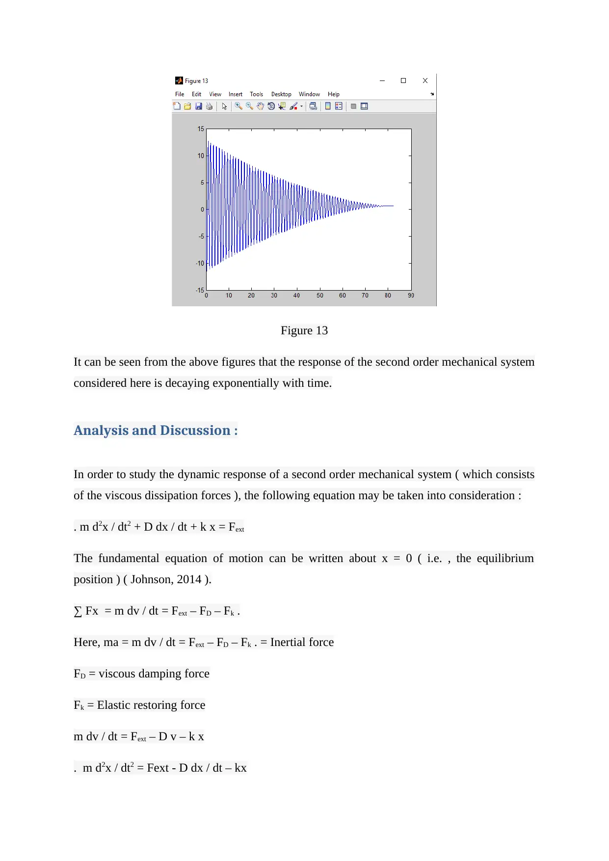
This report presents an analysis of a second-order mechanical system, focusing on its free and forced responses. The study utilizes a cart and two springs, and experiments are conducted using Capstone software at various voltage levels. Readings of position versus time are taken and plotted to analyze the system's behavior, including its transient response. The report examines the governing equation of motion, considering inertial, viscous damping, and elastic restoring forces. It explores the free response, considering different damping scenarios (underdamped, critically damped, and overdamped), and derives the relevant equations. Furthermore, the report investigates the forced response of the system. The results show the system's response decaying exponentially with time. The analysis includes references to relevant literature on system dynamics and mechanical systems.

Mechanical Engg.
SYSTEM DYNAMICS I
Abstract :
The exploration of the free and forced response of a second order mechanical system and the
estimation of the key parameters from the responses measured. The system dynamics
modelling as well as the transient and frequency responses are used for the same.
Procedure :
The mechanical system under study consists of a cart and 2 springs. The system is studied
using the Capstone software. The readings are taken at different voltage levels. The voltage
values chosen are : 4 V, 5 V, 6 V, 7 V, 9.43 V, 10 V, 11 V, 12 V and 13 V. The values are
taken at different time instants for the position in the unit of cm. The transient response is
also studied and the position value is noted at various instants of time. The values are
obtained in a text file. The readings are plotted and the graphs are studied.
Result :
The Figure 1 to 9 show the plot of position w.r.t. time for the voltage values chosen as : 4 V,
5 V, 6 V, 7 V, 9.43 V, 10 V, 11 V, 12 V and 13 V. The transient response is shown in Figure
10 to 13 which shows the position value is at various instants of time.

Figure 1
Figure 2

Figure 3
Figure 4

Figure 5
Figure 6

Figure 7
Figure 8

Figure 9
Figure 10

Figure 11
Figure 12

Figure 13
It can be seen from the above figures that the response of the second order mechanical system
considered here is decaying exponentially with time.
Analysis and Discussion :
In order to study the dynamic response of a second order mechanical system ( which consists
of the viscous dissipation forces ), the following equation may be taken into consideration :
. m d2x / dt2 + D dx / dt + k x = Fext
The fundamental equation of motion can be written about x = 0 ( i.e. , the equilibrium
position ) ( Johnson, 2014 ).
∑ Fx = m dv / dt = Fext – FD – Fk .
Here, ma = m dv / dt = Fext – FD – Fk . = Inertial force
FD = viscous damping force
Fk = Elastic restoring force
m dv / dt = Fext – D v – k x
. m d2x / dt2 = Fext - D dx / dt – kx

Here, v = dx / dt and ‘m’ is the equivalent mass, ‘D’ is the viscous damping coefficient and
‘k’ is the stiffness coefficient ( Zumalacárregui, 2014 ).
At t = 0, the initial conditions are :
. v ( 0 ) = v0 ( velocity ) and x ( 0 ) = x0 ( displacement ).
Free Response of Second Order Mechanical System
Here, the pure viscous damping forces are considered ( Peng, 2013 ). If the external force is 0
and the initial conditions for displacement and velocity are ( x0 , v0 ), then the equation of
motion is given by :
m d2x / dt2 + D dx / dt + kx = Fext
d2x / dt2 + D / m dx / dt + k x / m = 0
The natural frequency ( undamped ) of the system is wn = √ k / m
The viscous damping ratio = D / 2 √ k m
The equation is compared to m d2x / dt2 + 2 ξ wn dx / dt + wn2 x = 0
The solution is of the form given :
. x ( t ) = A est
A = constant ( determined using the initial conditions ) ( Li , 2016 )
Characteristic equation is : s2 + 2 ξ wn s + wn2 = 0
. x (t) = A1 es1t + A2 es2t
Here, s1 = - ξ wn + wn √ ξ 2 – 1
And s2 = - ξ wn - wn √ ξ 2 – 1
In under damped system, 0 < ξ < 1
x(t) = e – ξ wn t ( C1 cosh ( wd t ) + C2 sinh ( wd t ) ) ( Lee, 2012 ) where, wd = wn √ ξ 2 – 1 =
damped natural frequency

In critically damped system, ξ = 1 ,
X ( t ) = e –wn t ( C1 + t C2 )
In over damped system, ξ > 1
. x ( t ) = e – ξ wn t ( C1 cosh ( w’ t ) + C2 sinh ( w’ t ) )
Where , w’ = wn √ ξ 2 – 1
Undamped response may be given as :
X (t) = C1 cos ( wn t ) + C2 sin ( wn t )
Forced response of second order mechanical system :
The equation of motion is given by :
m d2x / dt2 + D dx / dt + kx = F
x(t)= A1 e s1 t + A2 e s2 t + F / k
A1 = A2 = constant
Undamped response :
x(t) = e – ξ wn t ( C1 cosh (wd t) + C2 sinh ( wd t ) ) + F0 / k
where, wd = wn √ ξ 2 – 1 = damped natural frequency
In over damped system, ξ > 1
. x(t) = e – ξ wn t ( C1 cosh ( w’ t ) + C2 sinh ( w’ t ) ) + Xss
Where , w’ = wn √ ξ 2 – 1 and Xss = F0 / k
In critically damped system, ξ = 1 ,
X(t) = e –wn t ( C1 + t C2 ) + Xss where Xss = F0 / k

Conclusions :
Hence, the second order mechanical system consisting of a cart and 2 springs has been
studied successfully. The response of the second order mechanical system has been found to
be decaying exponentially with time. The free response as well as the forced response has
been studied.
References :
Johnson, E., Schultz, J. and Murphey, T., 2014. Structured linearization of discrete
mechanical systems for analysis and optimal control. IEEE Transactions on Automation
Science and Engineering, 12(1), pp.140-152.
Lee, I., Noh, Y. and Yoo, D., 2012. A novel second-order reliability method (SORM) using
noncentral or generalized chi-squared distributions. Journal of Mechanical Design, 134(10).
Li, Z.H., Ma, Q. and Cui, J., 2016. Second-order two-scale finite element algorithm for
dynamic thermo–mechanical coupling problem in symmetric structure. Journal of
Computational Physics, 314, pp.712-748.
Peng, Q., Wen, X. and De, S., 2013. Mechanical stabilities of silicene. Rsc Advances, 3(33),
pp.13772-13781.
Zumalacárregui, M. and García-Bellido, J., 2014. Transforming gravity: from derivative
couplings to matter to second-order scalar-tensor theories beyond the Horndeski
Lagrangian. Physical Review D, 89(6), p.064046.