Introduction to Regression Analysis

This document provides an introduction to regression analysis and includes solved assignments and essays for the MGEC11H3S course. It covers topics such as regression summary, coefficients, significance tests, and regression equations.

Running Head: MGEC11H3S INTRODUCTION TO REGRESSION ANALYSIS
MGEC11H3S Introduction to Regression Analysis
Name of the Student
Name of the University
Student ID

1MGEC11H3S INTRODUCTION TO REGRESSION ANALYSIS
Table of Contents
2019-03-22 Assignment Data BENEFITS.................................................................................2
Answer 1................................................................................................................................2
Answer 2................................................................................................................................2
Answer 3................................................................................................................................3
Answer 4................................................................................................................................3
Answer 5................................................................................................................................4
Answer 6................................................................................................................................4
Answer 7................................................................................................................................4
2019-03-22 Assignment Data BEAUTY...................................................................................5
Answer 8................................................................................................................................5
Answer 9................................................................................................................................5
Answer 10..............................................................................................................................5
Answer 11..............................................................................................................................6
Answer 12..............................................................................................................................6
Answer 13..............................................................................................................................6
Answer 14..............................................................................................................................6
Answer 15..............................................................................................................................7

2MGEC11H3S INTRODUCTION TO REGRESSION ANALYSIS
2019-03-22 Assignment Data BENEFITS
Answer 1
Regression Summary of lavgsal on bs
Regression Statistics
Multiple R 0.070
R Square 0.005
Adjusted R
Square 0.004
Standard
Error 0.232
Observations 1848
ANOVA
df SS MS F
Significanc
e F
Regression 1 0.496 0.496 9.182 0.002
Residual 1846 99.686 0.054
Total 1847 100.181
Coefficients
Standard
Error t Stat
P-
value Lower 95%
Upper
95%
Intercept 10.648 0.057 186.018 0.000 10.535 10.760
bs -0.503 0.166 -3.030 0.002 -0.829 -0.178
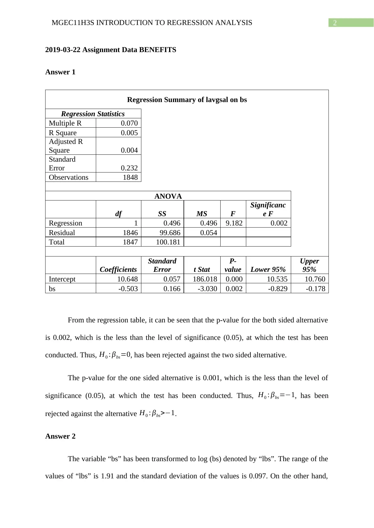
From the regression table, it can be seen that the p-value for the both sided alternative
is 0.002, which is the less than the level of significance (0.05), at which the test has been
conducted. Thus, H0 : βbs=0, has been rejected against the two sided alternative.
The p-value for the one sided alternative is 0.001, which is the less than the level of
significance (0.05), at which the test has been conducted. Thus, H0 : βbs=−1, has been
rejected against the alternative H0 : βbs>−1.
Answer 2
The variable “bs” has been transformed to log (bs) denoted by “lbs”. The range of the
values of “lbs” is 1.91 and the standard deviation of the values is 0.097. On the other hand,

3MGEC11H3S INTRODUCTION TO REGRESSION ANALYSIS
the range and standard deviation of “bs” has been found to be 0.56 and 0.033 respectively.
Thus, it can be said that the variation in the values of “bs” is less than that of the values in
“lbs”.
Answer 3
Regression Summary of lavgsal on lbs
Regression Statistics
Multiple R 0.063
R Square 0.004
Adjusted R
Square 0.003
Standard Error 0.233
Observations 1848
ANOVA
df SS MS F
Significance
F
Regression 1 0.391 0.391 7.241 0.007
Residual 1846 99.790 0.054
Total 1847 100.181
Coefficie
nts
Standard
Error t Stat
P-
value Lower 95%
Upper
95%
Intercept 10.313 0.060
171.06
2 0.000 10.195 10.432
lbs -0.150 0.056 -2.691 0.007 -0.260 -0.041
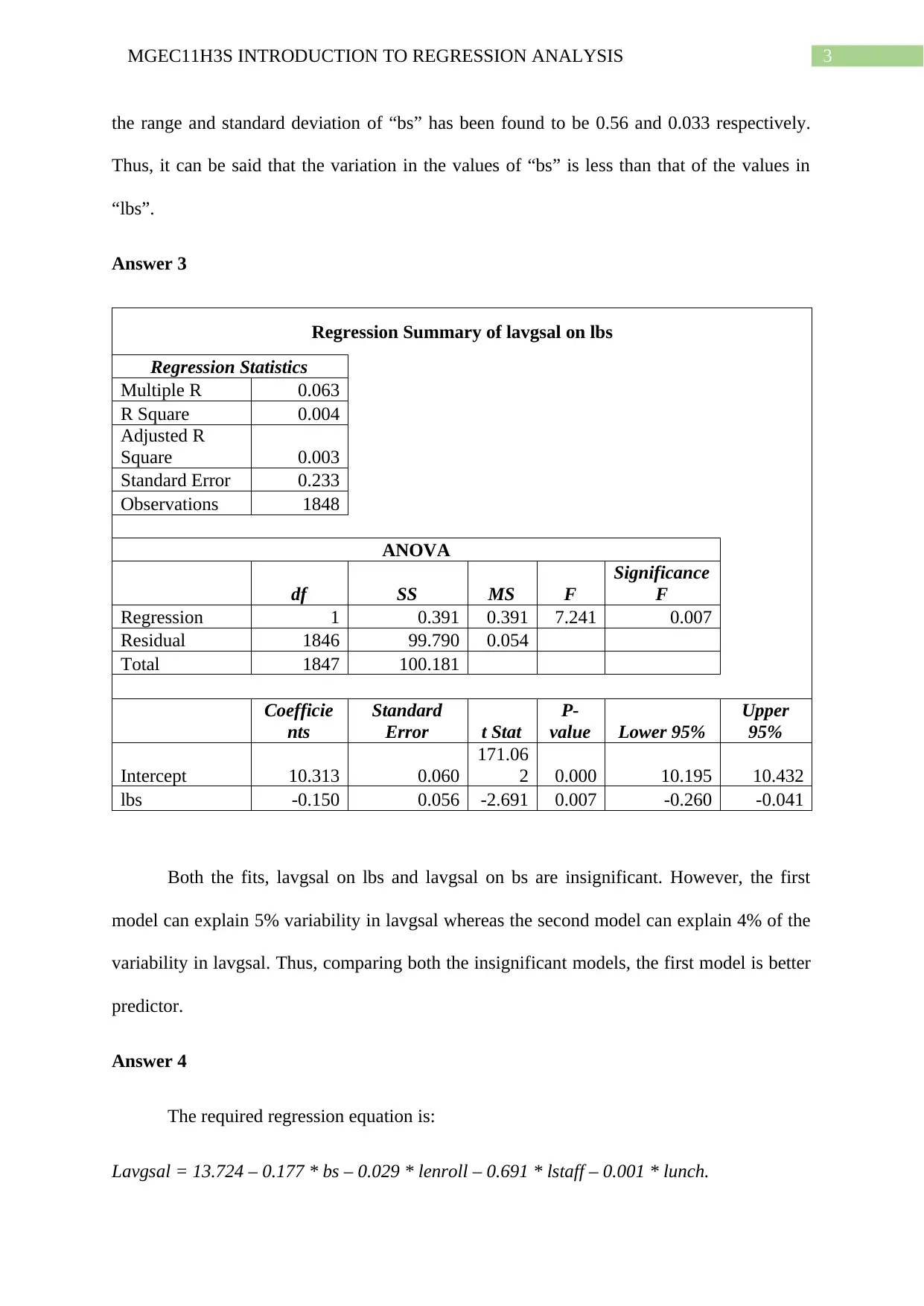
Both the fits, lavgsal on lbs and lavgsal on bs are insignificant. However, the first
model can explain 5% variability in lavgsal whereas the second model can explain 4% of the
variability in lavgsal. Thus, comparing both the insignificant models, the first model is better
predictor.
Answer 4
The required regression equation is:
Lavgsal = 13.724 – 0.177 * bs – 0.029 * lenroll – 0.691 * lstaff – 0.001 * lunch.

4MGEC11H3S INTRODUCTION TO REGRESSION ANALYSIS
It can be seen in this model that the p-value for the variable bs is 0.146, which is
higher than the level of significance (0.05). thus, the variable bs has now become statistically
significant to the model.
Answer 5
In the model developed in the previous question, it can be seen that the coefficient of
the variable lstaff is – 0.691. This indicates that for each unit increase in the log of the
number of staffs per 1000 students, the log of the average salary of teacher decreases. The
coefficient of the variable lstaff is negative as if the number of students remain constant and
the number of teachers increase, then the salary of the teachers will decrease.
Answer 6
The variable lunch2 has been found to be statistically insignificant and the value of the
coefficient has also been found to be negligible. Thus, there is no quadratic form to the model
to be calculating the turning point.
Answer 7
Keeping all the other factors constant, when lunch = 0 (no poverty), the salary of the
teachers is the maximum. With the increase in the value of lunch, the salary decreases. Thus,
it is better to work in a school with no poverty.

5MGEC11H3S INTRODUCTION TO REGRESSION ANALYSIS
2019-03-22 Assignment Data BEAUTY
Answer 8
Gender Above Average Looks Grand Total
0 1
0 0.46 0.19 0.65
1 0.23 0.11 0.35
Grand Total 0.70 0.30 1
From the table, it can be seen that more people rated as having below average looks.
Answer 9
A simple linear regression has been conducted to test whether the population fractions
of above average looking women and men are the same. It can be said from the regression
results that p-value for the model is 0.140, which is higher than the level of significance
(0.05), at which the test has been conducted. Thus, it can be said that there is no significant
difference in the proportion of above average looking men and women.
Answer 10
For male, the estimated model is given by:
Log (wage) = 1.884 – 0.199 * belavg – 0.044 * abvavg
It can be said from the regression equation that the wage of below average men
decreases by 0.199. The p-value for men is 0.001. This indicates that the log (wage) of men is
not significantly affected by their below average looks.
For female, the estimated model is given by:
Log (wage) = 1.309 – 0.138 * belavg + 0.034 * abvavg

6MGEC11H3S INTRODUCTION TO REGRESSION ANALYSIS
It can be said from the regression equation that the wage of below average women
decreases by 0.138. The p-value for women is 0.072. This indicates that the log (wage) of
women are significantly affected by their below average looks.
Answer 11
A simple linear regression has been conducted to test whether women with above
average looks earn more than women with average looks. From the results of the regression
analysis, it can be seen that the p-value of the model is 0.154, which is greater than the level
of significance (0.05), at which the test has been conducted. Further, the regression
coefficient of the variable (0.596) is also positive. Thus, it can be said from here that women
with above average looks earn more than women with average looks.
Answer 12
The first model has been conducted without the introduction of the variable “looks”.
The second model on the other hand has been constructed with “looks” as an explanatory
variable. In both the cases, the estimated model has been found to be significant. Introduction
of the variable “looks” has not made any significant effect in the two different models.
Answer 13
lwage= 0.559
( 0.080 ) −0.154 ×belavg
( 0.042 ) −0.007 × abvavg
( 0.031 ) −0.453× female
( 0.029 ) +0.066 × educ
( 0.005 ) + 0.041× exper
( 0.004 ) −0.001× expe
( 0.005 )
It can be seen from here that the coefficient for female is comparatively large and is
also statistically significant as p-value is less than 0.05.
Answer 14

7MGEC11H3S INTRODUCTION TO REGRESSION ANALYSIS
The value of the F-test of significance without the interaction effects has been found
to be 117.356, whereas with the inclusion of the interaction variables it has been found to be
66.193. Thus, it can be seen that values of the F-test for the two different models differ a lot.
Answer 15
The interaction effects of female with the looks variables, female×belavg and
female×abvavg hav been found to be statistically insignificant in the model due to higher p-
values. Their coefficients are also practically small.