Northcutt Bikes Supply Chain Management Essentials

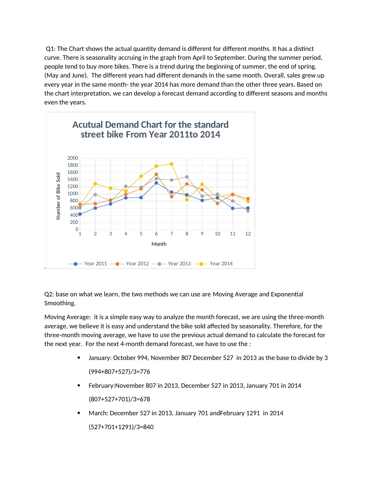
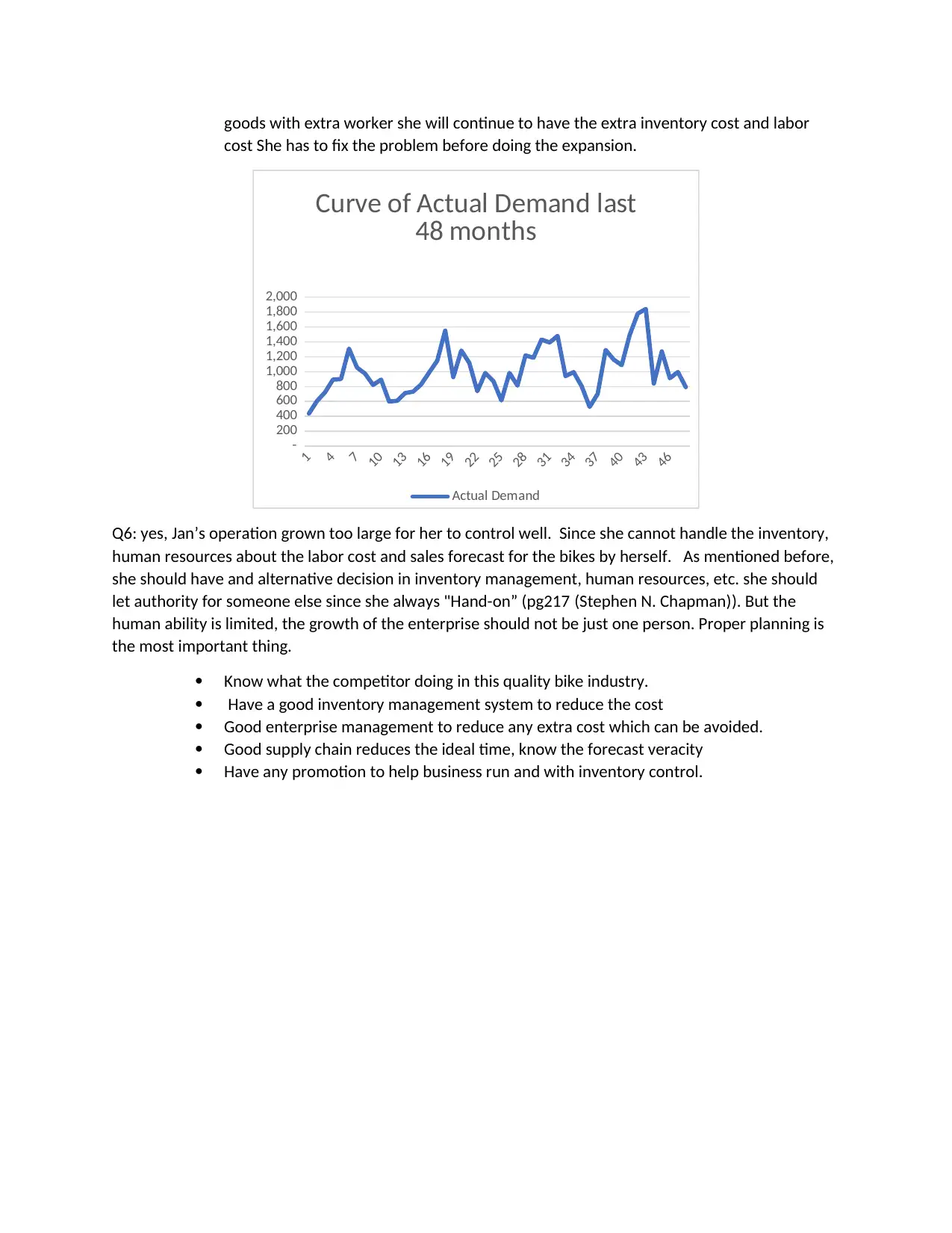
This assignment involves analyzing the supply chain management essentials of Northcutt Bikes, specifically focusing on forecasting demand using moving average and exponential smoothing methods. The goal is to ensure effective inventory management, reducing costs and ideal time. The student must consider Jan's knowledge and ability in managing her business, including controlling expansion, understanding competitor activity, and implementing good enterprise management practices.

MGT2314 supply chain management essentials
Case Study 2-Northcut Bikes

Q1: The Chart shows the actual quantity demand is different for different months. It has a distinct
curve. There is seasonality accruing in the graph from April to September. During the summer period,
people tend to buy more bikes. There is a trend during the beginning of summer, the end of spring.
(May and June). The different years had different demands in the same month. Overall, sales grew up
every year in the same month- the year 2014 has more demand than the other three years. Based on
the chart interpretation, we can develop a forecast demand according to different seasons and months
even the years.
.
1 2 3 4 5 6 7 8 9 10 11 12
0
200
400
600
800
1000
1200
1400
1600
1800
2000
Acutual Demand Chart for the standard
street bike From Year 2011to 2014
Year 2011 Year 2012 Year 2013 Year 2014
Month
Number of Bike Sold
Q2: base on what we learn, the two methods we can use are Moving Average and Exponential
Smoothing.
Moving Average: it is a simple easy way to analyze the month forecast, we are using the three-month
average, we believe it is easy and understand the bike sold affected by seasonality. Therefore, for the
three-month moving average, we have to use the previous actual demand to calculate the forecast for
the next year. For the next 4-month demand forecast, we have to use the :
 January: October 994, November 807 December 527 in 2013 as the base to divide by 3
(994+807+527)/3=776
 February:November 807 in 2013, December 527 in 2013, January 701 in 2014
(807+527+701)/3=678
 March: December 527 in 2013, January 701 andFebruary 1291 in 2014
(527+701+1291)/3=840

 April: January 701, February 1291, March 1162 base in 2014
( 701+1291+1162)/3=1052
Therefore, using the three-month moving average method to forecast the next four-month demand is
776,678, 840 and 1052.
Exponential Smoothing: in this case, according to the data analysis, its rate of change is relatively not
large, base on which, we assume the value of alpha to 0.2 and set the December year 2013 forecast is
800. Use the formula: New forecast= (a) (latest demand) + (1-a) (previous forecast) (Forecasting and
Demand Management , 2017)we can get forecast is:
January =0.2 *792 +0.8*800=798.4=799
February: 0.2 *701+ 0.8*799=779.4=780
March: 0.2*1291+0.8*780=882
April: 0.2*1162+ 0.8*882=938
Using the assume data, we can the forecast for next three month is 799,780,882 and 938.
There are many other methods to forecast the demand, such as we can average four years’ January
demand to get the forecast for 2015, using the 12-month average to calculate the forecast as well.
Q3: Base on the above two sets of forecast numbers, and compared with the previous three years of
data. A better way is to have a month moving average. Three months of numbers can be used to identify
the recent demand without too much error. The other way is because we assumed an alpha and we
assumed a predictive value it is kind of has a limitation, we don’t have mean absolute Deviation (MAD)
to analyze. Therefore, we get a relatively small quantity demanded of the exponential smoothing
method. month moving average method is better.
Q4: Base on Jan's knowledge and ability, we should know that the bicycle is limited. Usually not suitable
in the winter, and people will ride it in the summer season. So, our forecast should be based on
quarterly. According to the Graph showed, the curve for the first half of the year is almost always rising
slowly although there is a gap. So, it is still going to grow up and then after summer, we see that
demand is going to down. This method will bring the overall data. For example, we a sales promotion or
kind of race. This will affect the sale of bicycles if only using the month, the forecast often not enough.
Q5: Base on the Data of the last 48-month curve and compare with Jan’s situation. She should not just
focus on the sales forecast she also can
 Inventory Management, since Jan has a big issue on her inventory such as reworking,
inventory not right situation, idle time. She should have a good plan to work in her
inventory system. It could help her to reduce the cost, and know the real customer
demand.
 Control the expansion: as her know her business is growing up rapidity, but she has to
focus on more the size since she doing very well on the quality because she makes her
bike on herself. She still needs to know about the competitive existence. if keep build

goods with extra worker she will continue to have the extra inventory cost and labor
cost She has to fix the problem before doing the expansion.
1
4
7
10
13
16
19
22
25
28
31
34
37
40
43
46
-
200
400
600
800
1,000
1,200
1,400
1,600
1,800
2,000
Curve of Actual Demand last
48 months
Actual Demand
Q6: yes, Jan’s operation grown too large for her to control well. Since she cannot handle the inventory,
human resources about the labor cost and sales forecast for the bikes by herself. As mentioned before,
she should have and alternative decision in inventory management, human resources, etc. she should
let authority for someone else since she always "Hand-on” (pg217 (Stephen N. Chapman)). But the
human ability is limited, the growth of the enterprise should not be just one person. Proper planning is
the most important thing.
 Know what the competitor doing in this quality bike industry.
 Have a good inventory management system to reduce the cost
 Good enterprise management to reduce any extra cost which can be avoided.
 Good supply chain reduces the ideal time, know the forecast veracity
 Have any promotion to help business run and with inventory control.

References
Forecasting and Demand Management . (2017). In J. R. Stephen N. Chapman, Introduction to Materials
Management (p. 199). Boston Columbus Indianapolis New York San Francisco Amsterdam :
Pearson.
Hayes, A. (2020, March 31). Moving Average. Retrieved from Inestopedia:
https://www.investopedia.com/terms/m/movingaverage.asp
Stephen N. Chapman, J. R. (n.d.). Case Study - Northcutt Bikes. In Introduction to Materials Management
(p. 2017). Boston Columbus Indianapolis New York San Francisco: Pearson.