Microeconomics 12: Analysis of Production, Taxes, and Disasters
VerifiedAdded on 2021/05/31
|12
|1939
|118
Homework Assignment
AI Summary
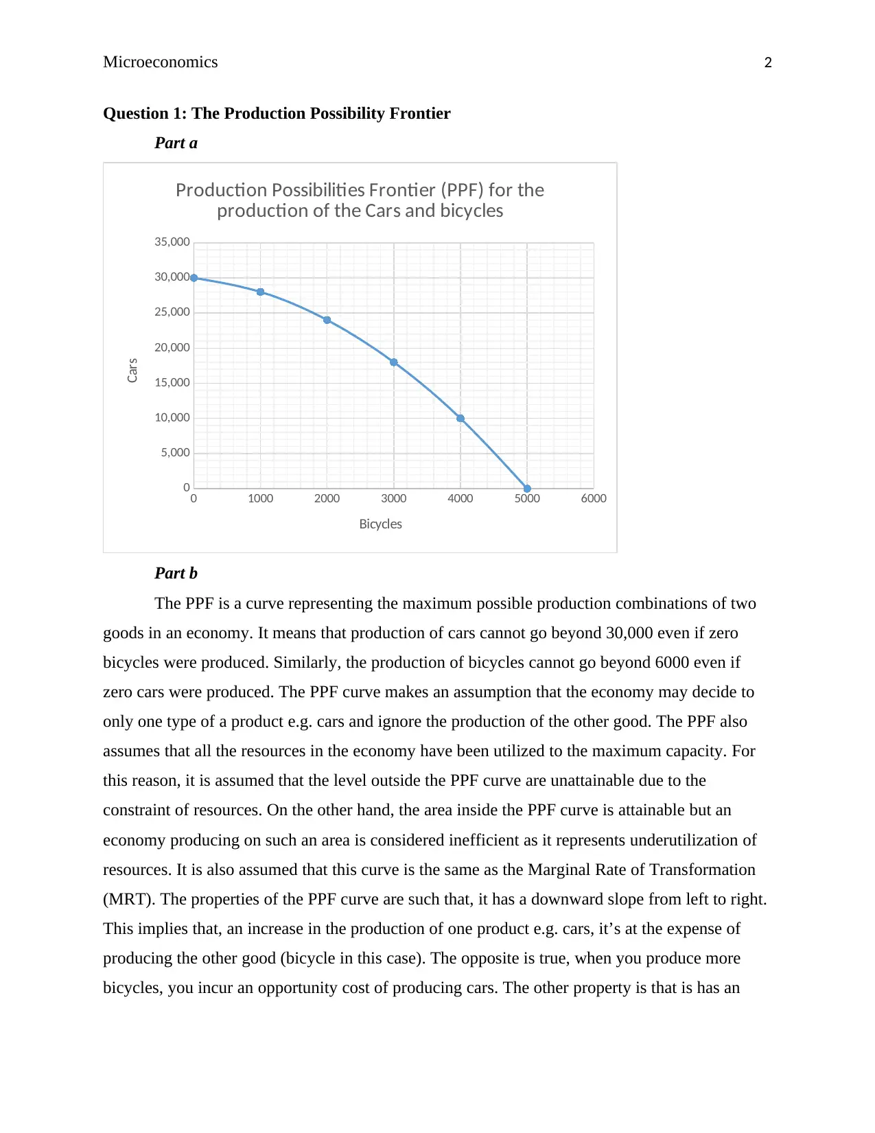
This microeconomics assignment analyzes several key economic concepts. The first question explores the Production Possibility Frontier (PPF), discussing its properties, attainable and unattainable combinations, and opportunity costs. The second question delves into tax incidence, calculating equilibrium, elasticity, and the burden of a per-unit tax on consumers and producers, including a graphical representation. The third question examines price regulation, specifically minimum price controls, analyzing oversupply, deadweight loss, and fairness of outcomes. The final question investigates the impact of a natural disaster on coffee supply, illustrating shifts in supply and demand, price changes, and market shortages, including graphical representations.
1 out of 12
Related Documents


Your All-in-One AI-Powered Toolkit for Academic Success.
+13062052269
info@desklib.com
Available 24*7 on WhatsApp / Email
![[object Object]](/_next/static/media/star-bottom.7253800d.svg)
Copyright © 2020–2026 A2Z Services. All Rights Reserved. Developed and managed by ZUCOL.