Microeconomic Analysis

This document provides a detailed analysis of microeconomics, covering topics such as supply and demand, market equilibrium, barriers to entry, and cost curves. It includes examples and explanations to help readers understand these concepts. The document also discusses the market structure of the fast food restaurant industry as an example of oligopoly.

Running head: Microeconomic Analysis
Microeconomic Analysis
Name of the Student
Name of the University
Student ID

1Microeconomic Analysis
Table of Contents
Answer 1..........................................................................................................................................2
Answer 2..........................................................................................................................................6
Answer 3..........................................................................................................................................7
Answer 4..........................................................................................................................................9
References......................................................................................................................................11

2Microeconomic Analysis
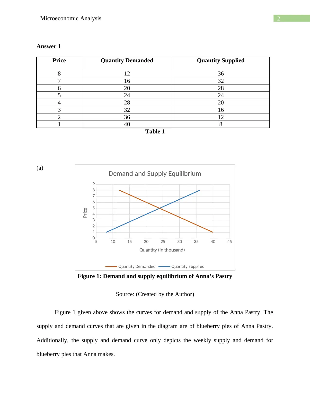
Answer 1
Price Quantity Demanded Quantity Supplied
8 12 36
7 16 32
6 20 28
5 24 24
4 28 20
3 32 16
2 36 12
1 40 8
Table 1
(a)
Figure 1: Demand and supply equilibrium of Anna’s Pastry
Source: (Created by the Author)
Figure 1 given above shows the curves for demand and supply of the Anna Pastry. The
supply and demand curves that are given in the diagram are of blueberry pies of Anna Pastry.
Additionally, the supply and demand curve only depicts the weekly supply and demand for
blueberry pies that Anna makes.
5 10 15 20 25 30 35 40 45
0
1
2
3
4
5
6
7
8
9
Demand and Supply Equilibrium
Quantity Demanded Quantity Supplied
Quantity (in thousand)
Price

3Microeconomic Analysis
(b)
The equilibrium price is the price for which the amount of blueberry supplied matches the
amount of blueberry demanded. Any deviation from that price will break the equality between
supply and demand (Azevedo and Leshno 2016). From microeconomic theory it is known that
price and supply are directly proportional and it means with rise in price, supply rises and vice
versa. On the other hand, demand and price are inversely associated and it means with rise in
price, demand declines and vice versa. These relationship can be observed in table 1, where with
surge in price demand declines and supply increases. The demand curve is downward sloping
due the converse relationship with price and supply curve is upward sloping due to positive
relationship with price (Friedman 2017). In table 1 it can be observed that at price 5 the
demanded quantity is 24000 and supplied quantity is also 24000. Thus, it is clear that at price 5
supply and demand for blueberry pies equalizes (Glasserman and Nouri 2016). Consequently, the
equilibrium quantity and price traded are 5 unit and 24000 respectively. In the figure 1, at
equilibrium quantity and price, the demand curve and supply curve intersects each other and thus
this intersection point is called market equilibrium point.

4Microeconomic Analysis
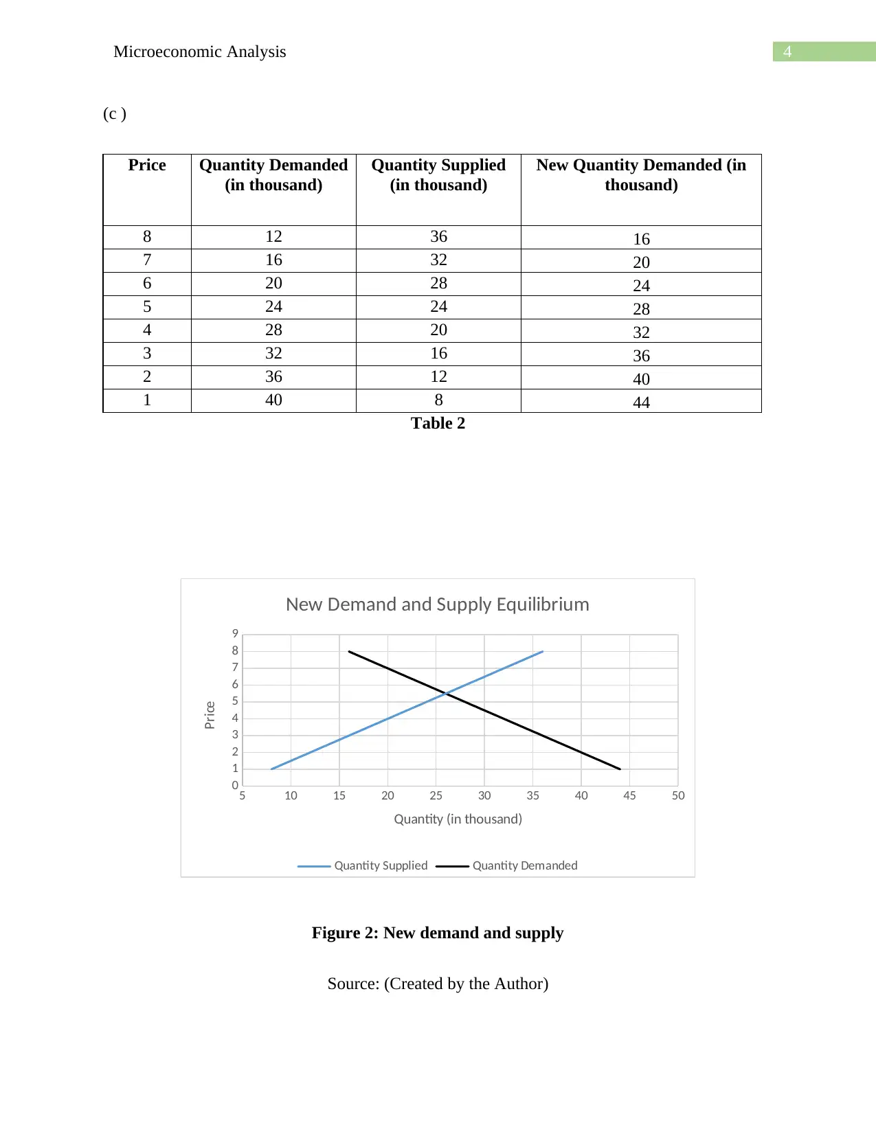
(c )
Price Quantity Demanded
(in thousand)
Quantity Supplied
(in thousand)
New Quantity Demanded (in
thousand)
8 12 36 16
7 16 32 20
6 20 28 24
5 24 24 28
4 28 20 32
3 32 16 36
2 36 12 40
1 40 8 44
Table 2
Figure 2: New demand and supply
Source: (Created by the Author)
5 10 15 20 25 30 35 40 45 50
0
1
2
3
4
5
6
7
8
9
New Demand and Supply Equilibrium
Quantity Supplied Quantity Demanded
Quantity (in thousand)
Price

5Microeconomic Analysis
In table 2 the new quantity demanded column shows the amount of demand for the
blueberry pies per week after increment in the quantity demanded for the same by 4000 units. In
figure 2 the new demand curve that is obtained after increase in demand for blueberry pies by
4000 units is given by black downward sloping demand curve.
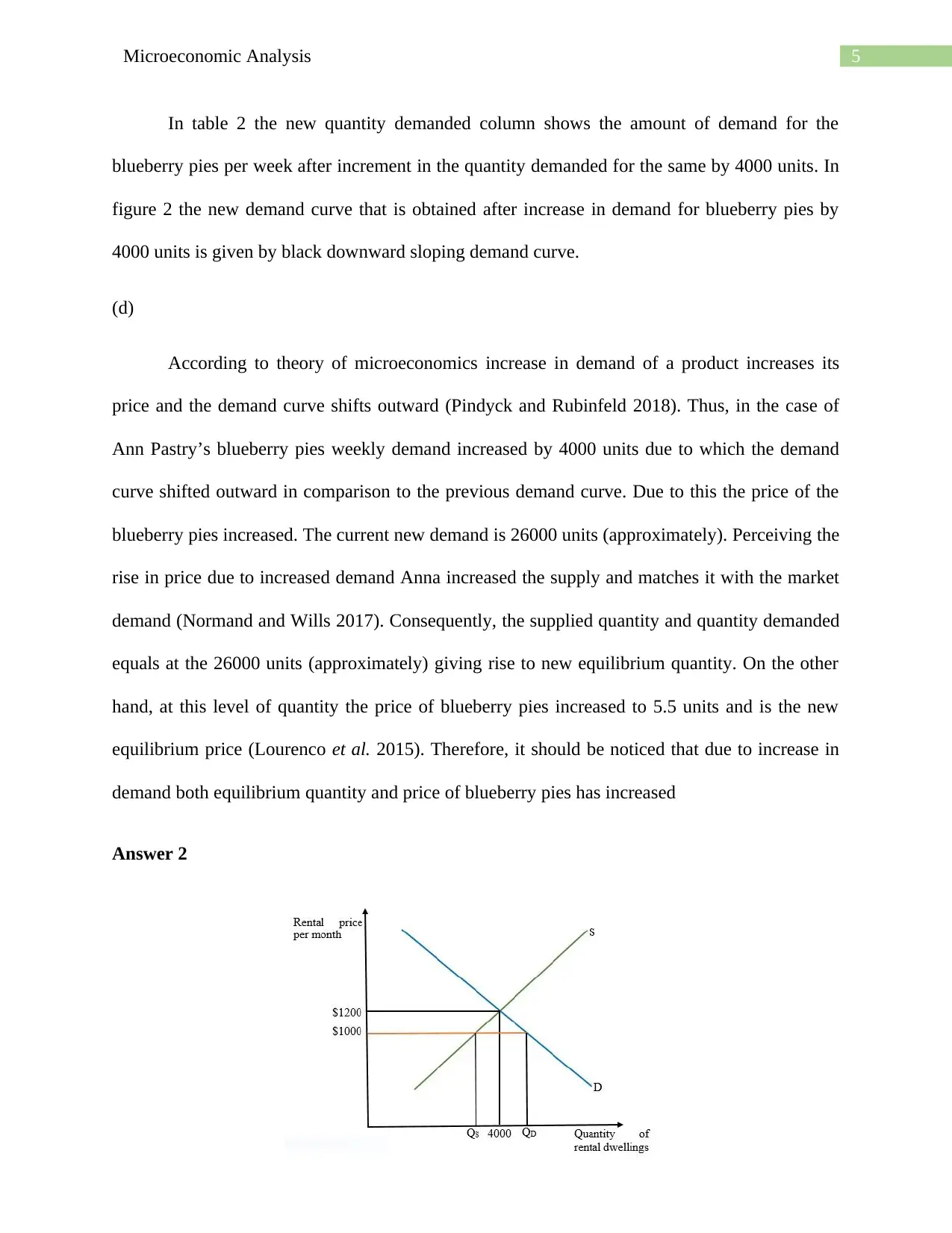
(d)
According to theory of microeconomics increase in demand of a product increases its
price and the demand curve shifts outward (Pindyck and Rubinfeld 2018). Thus, in the case of
Ann Pastry’s blueberry pies weekly demand increased by 4000 units due to which the demand
curve shifted outward in comparison to the previous demand curve. Due to this the price of the
blueberry pies increased. The current new demand is 26000 units (approximately). Perceiving the
rise in price due to increased demand Anna increased the supply and matches it with the market
demand (Normand and Wills 2017). Consequently, the supplied quantity and quantity demanded
equals at the 26000 units (approximately) giving rise to new equilibrium quantity. On the other
hand, at this level of quantity the price of blueberry pies increased to 5.5 units and is the new
equilibrium price (Lourenco et al. 2015). Therefore, it should be noticed that due to increase in
demand both equilibrium quantity and price of blueberry pies has increased
Answer 2

6Microeconomic Analysis
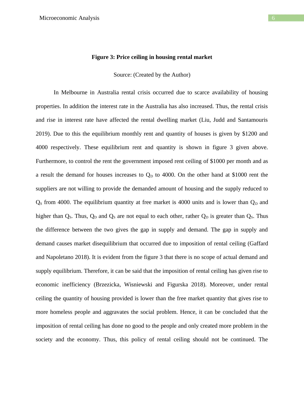
Figure 3: Price ceiling in housing rental market
Source: (Created by the Author)
In Melbourne in Australia rental crisis occurred due to scarce availability of housing
properties. In addition the interest rate in the Australia has also increased. Thus, the rental crisis
and rise in interest rate have affected the rental dwelling market (Liu, Judd and Santamouris
2019). Due to this the equilibrium monthly rent and quantity of houses is given by $1200 and
4000 respectively. These equilibrium rent and quantity is shown in figure 3 given above.
Furthermore, to control the rent the government imposed rent ceiling of $1000 per month and as
a result the demand for houses increases to QD to 4000. On the other hand at $1000 rent the
suppliers are not willing to provide the demanded amount of housing and the supply reduced to
QS from 4000. The equilibrium quantity at free market is 4000 units and is lower than QD and
higher than QS. Thus, QD and QS are not equal to each other, rather QD is greater than QS. Thus
the difference between the two gives the gap in supply and demand. The gap in supply and
demand causes market disequilibrium that occurred due to imposition of rental ceiling (Gaffard
and Napoletano 2018). It is evident from the figure 3 that there is no scope of actual demand and
supply equilibrium. Therefore, it can be said that the imposition of rental ceiling has given rise to
economic inefficiency (Brzezicka, Wisniewski and Figurska 2018). Moreover, under rental
ceiling the quantity of housing provided is lower than the free market quantity that gives rise to
more homeless people and aggravates the social problem. Hence, it can be concluded that the
imposition of rental ceiling has done no good to the people and only created more problem in the
society and the economy. Thus, this policy of rental ceiling should not be continued. The

7Microeconomic Analysis
determination of equilibrium price and quantity of the housing market is thus left to the free
market forces to achieve more welfare.
Answer 3
In order to enter a fast food restaurant industry a firm needs to invest significant sum of
money as opening several branches, hiring cooks and purchase of cooking equipment require
considerable amount of investment. Apart, from that the exiting big companies will restrict entry
of new firms by intense pricing strategies. Thus in this industry there exists barriers to entry. This
industry is dominated by KFC, McDonalds, Hungry Jacks and Dominos Pizza (Nguyen and Wait
2015). There are few firms in the business and a large number of buyers. The companies that are
present in the market are all big players and they dominate the market. Thus, the firms have
significant market power and they can charge high price to gain profit above normal profit level.
In this industry the player or the firms serve same category of food. Therefore, there is no
uniqueness in product like in the case of monopoly market but as the production of food is
expensive that makes it difficult for other firms to produce it. Additionally, huge fixed cost is
associated with the industry and thus if a firm decides to make an exit then it has to bear the loss
of fixed cost. Moreover, as there are low number of firms exit of any of them will affect the
supply and price of the products in the industry (Polutnik 2015). The customers in this restaurant
industry are price takers and thus get exploited when they are charged with high price. In case, of
KFC the target group of customers are those who prefers fried chicken dishes, for McDonalds
the target customer are those who love to consume burgers. Similarly, for Dominos Pizza the
target group of customer are the ones who prefer to consume pizza. All these are part of
restaurant industry and the companies mentioned above can replicate the model of the other
easily. Hence, even after serving different food products all these companies operate in the same

8Microeconomic Analysis
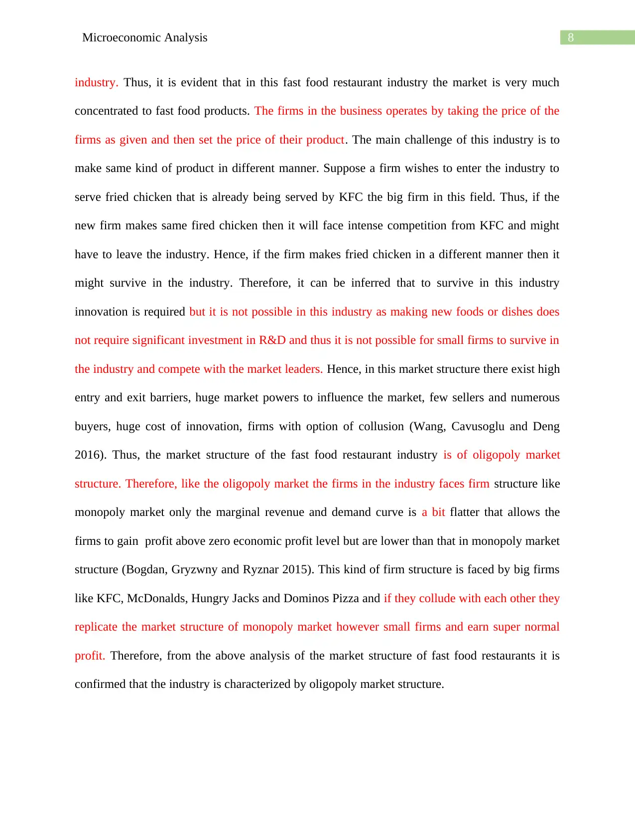
industry. Thus, it is evident that in this fast food restaurant industry the market is very much
concentrated to fast food products. The firms in the business operates by taking the price of the
firms as given and then set the price of their product. The main challenge of this industry is to
make same kind of product in different manner. Suppose a firm wishes to enter the industry to
serve fried chicken that is already being served by KFC the big firm in this field. Thus, if the
new firm makes same fired chicken then it will face intense competition from KFC and might
have to leave the industry. Hence, if the firm makes fried chicken in a different manner then it
might survive in the industry. Therefore, it can be inferred that to survive in this industry
innovation is required but it is not possible in this industry as making new foods or dishes does
not require significant investment in R&D and thus it is not possible for small firms to survive in
the industry and compete with the market leaders. Hence, in this market structure there exist high
entry and exit barriers, huge market powers to influence the market, few sellers and numerous
buyers, huge cost of innovation, firms with option of collusion (Wang, Cavusoglu and Deng
2016). Thus, the market structure of the fast food restaurant industry is of oligopoly market
structure. Therefore, like the oligopoly market the firms in the industry faces firm structure like
monopoly market only the marginal revenue and demand curve is a bit flatter that allows the
firms to gain profit above zero economic profit level but are lower than that in monopoly market
structure (Bogdan, Gryzwny and Ryznar 2015). This kind of firm structure is faced by big firms
like KFC, McDonalds, Hungry Jacks and Dominos Pizza and if they collude with each other they
replicate the market structure of monopoly market however small firms and earn super normal
profit. Therefore, from the above analysis of the market structure of fast food restaurants it is
confirmed that the industry is characterized by oligopoly market structure.

9Microeconomic Analysis
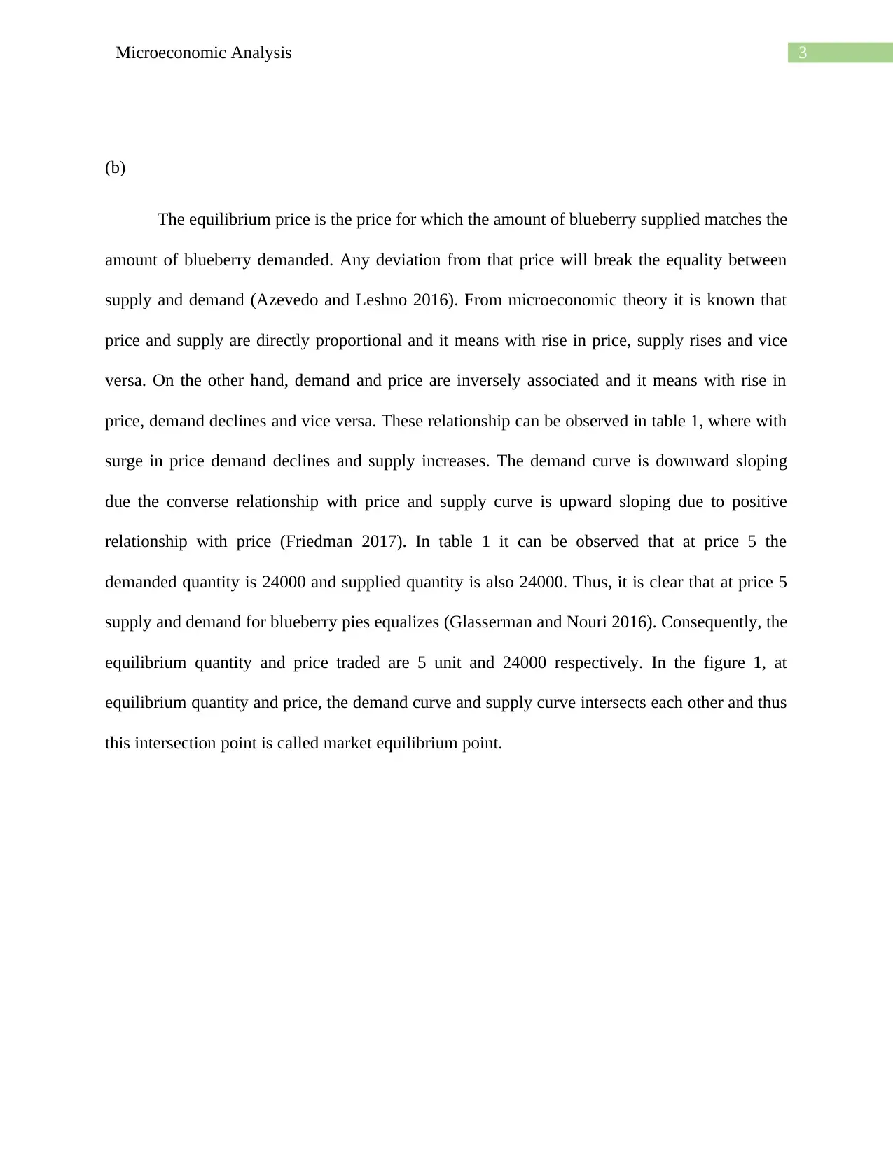
Answer 4
Table 3
.
Figure 4: Marginal cost and Average costs
Source: (Created by the Author)
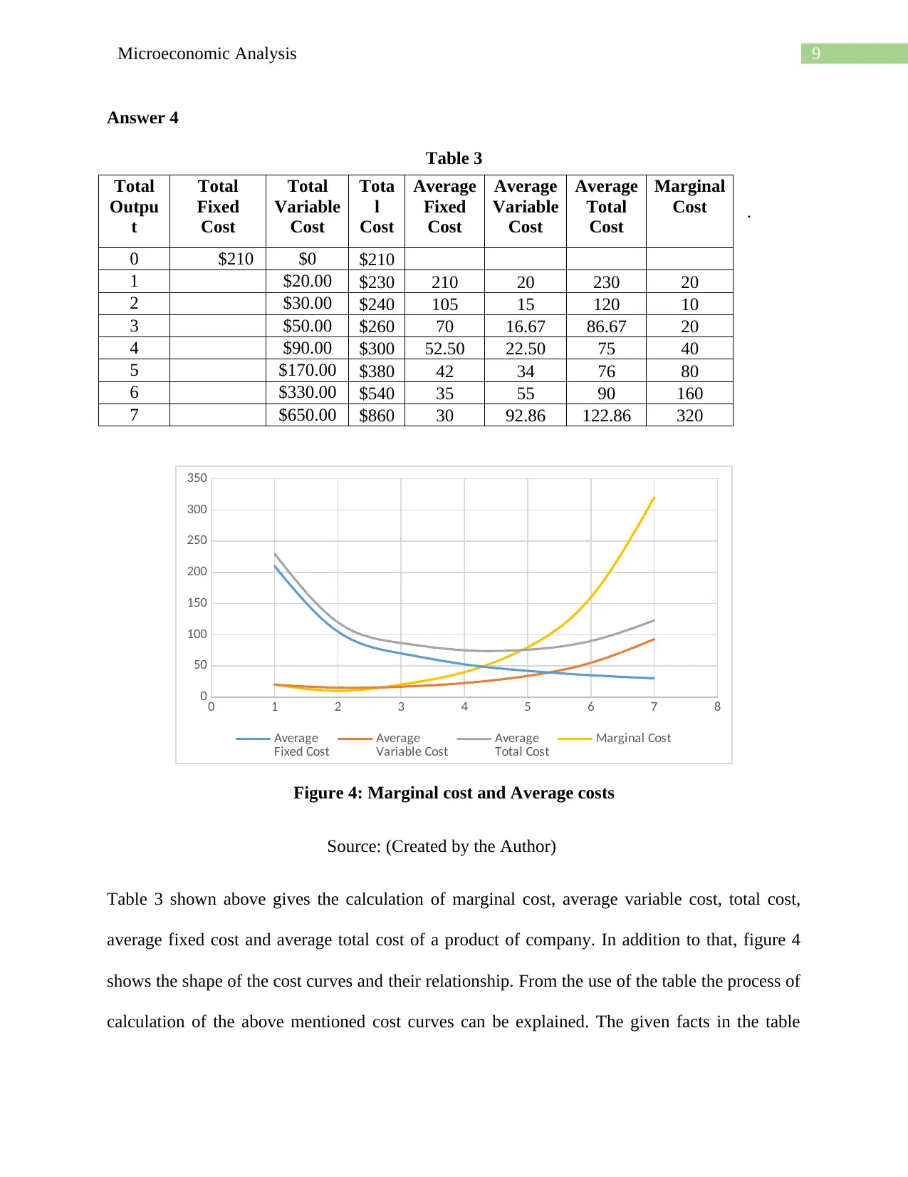
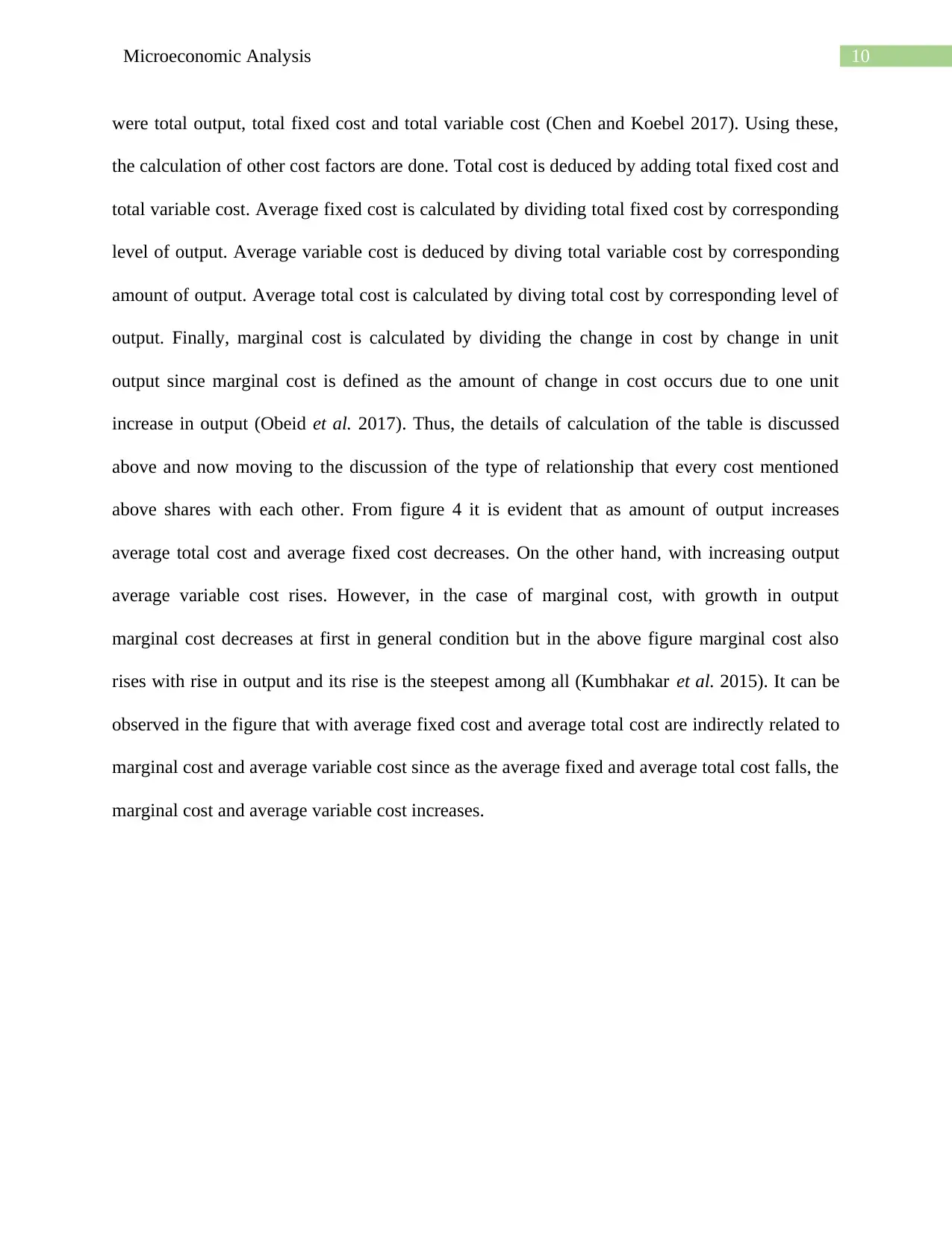
Table 3 shown above gives the calculation of marginal cost, average variable cost, total cost,
average fixed cost and average total cost of a product of company. In addition to that, figure 4
shows the shape of the cost curves and their relationship. From the use of the table the process of
calculation of the above mentioned cost curves can be explained. The given facts in the table
0 1 2 3 4 5 6 7 8
0
50
100
150
200
250
300
350
Average
Fixed Cost Average
Variable Cost Average
Total Cost Marginal Cost
Total
Outpu
t
Total
Fixed
Cost
Total
Variable
Cost
Tota
l
Cost
Average
Fixed
Cost
Average
Variable
Cost
Average
Total
Cost
Marginal
Cost
0 $210 $0 $210
1 $20.00 $230 210 20 230 20
2 $30.00 $240 105 15 120 10
3 $50.00 $260 70 16.67 86.67 20
4 $90.00 $300 52.50 22.50 75 40
5 $170.00 $380 42 34 76 80
6 $330.00 $540 35 55 90 160
7 $650.00 $860 30 92.86 122.86 320

10Microeconomic Analysis
were total output, total fixed cost and total variable cost (Chen and Koebel 2017). Using these,
the calculation of other cost factors are done. Total cost is deduced by adding total fixed cost and
total variable cost. Average fixed cost is calculated by dividing total fixed cost by corresponding
level of output. Average variable cost is deduced by diving total variable cost by corresponding
amount of output. Average total cost is calculated by diving total cost by corresponding level of
output. Finally, marginal cost is calculated by dividing the change in cost by change in unit
output since marginal cost is defined as the amount of change in cost occurs due to one unit
increase in output (Obeid et al. 2017). Thus, the details of calculation of the table is discussed
above and now moving to the discussion of the type of relationship that every cost mentioned
above shares with each other. From figure 4 it is evident that as amount of output increases
average total cost and average fixed cost decreases. On the other hand, with increasing output
average variable cost rises. However, in the case of marginal cost, with growth in output
marginal cost decreases at first in general condition but in the above figure marginal cost also
rises with rise in output and its rise is the steepest among all (Kumbhakar et al. 2015). It can be
observed in the figure that with average fixed cost and average total cost are indirectly related to
marginal cost and average variable cost since as the average fixed and average total cost falls, the
marginal cost and average variable cost increases.

11Microeconomic Analysis
References
Azevedo, E.M. and Leshno, J.D., 2016. A supply and demand framework for two-sided
matching markets. Journal of Political Economy, 124(5), pp.1235-1268.
Bogdan, K., Grzywny, T. and Ryznar, M., 2015. Barriers, exit time and survival probability for
unimodal Lévy processes. Probability Theory and Related Fields, 162(1-2), pp.155-198.
Brzezicka, J., Wisniewski, R. and Figurska, M., 2018. Disequilibrium in the real estate market:
Evidence from Poland. Land use policy, 78, pp.515-531.
Chen, X. and Koebel, B.M., 2017. Fixed cost, variable cost, markups and returns to
scale. Annals of Economics and Statistics/Annales d'Économie et de Statistique, (127), pp.61-94.
Friedman, M., 2017. Price theory. Routledge.
Gaffard, J.L. and Napoletano, M., 2018. Market disequilibrium, monetary policy, and Financial
markets: Insights from new tools (No. 2018/17). LEM Working Paper Series.
Glasserman, P. and Nouri, B., 2016. Market‐triggered changes in capital structure: Equilibrium
price dynamics. Econometrica, 84(6), pp.2113-2153.
Kumbhakar, S., Parmeter, C., Stefanou, S. and Lansink, A.O., 2015. THEORY AND PRACTICE
OF EFFICIENCY & PRODUCTIVITY MEASUREMENT: STATIC & DYNAMIC
ANALYSIS (Doctoral dissertation, Universidad Santo Tomas, Chile).
Liu, E., Judd, B. and Santamouris, M., 2019. Challenges in transitioning to low carbon living for
lower income households in Australia. Advances in Building Energy Research, 13(1), pp.49-64.

12Microeconomic Analysis
Lourenço, T.C., Swart, R., Goosen, H. and Street, R., 2015. The rise of demand-driven climate
services. Nature Climate Change, 6(1), p.13.
Nguyen, B. and Wait, A., 2015. Essentials of Microeconomics. Routledge.
Norman, S. and Wills, D., 2017. The Importance of Emphasizing the Intertemporal Consumption
Model in Intermediate Microeconomics. Journal for Economic Educators, 17(1), pp.25-29.
Obeid, T., Alshaikh, H., Nejim, B., Arhuidese, I., Locham, S. and Malas, M., 2017. Fixed and
variable cost of carotid endarterectomy and stenting in the United States: a comparative
study. Journal of vascular surgery, 65(5), pp.1398-1406.
Pindyck, R.S. and Rubinfeld, D.L., 2018. Microeconomics (Global ed., The Pearson series in
economics). Harlow: Pearson.
Polutnik, L., 2015. Total Variable Cost. Wiley Encyclopedia of Management, pp.1-1.
Wang, S., Cavusoglu, H. and Deng, Z., 2016. Early mover advantage in e-commerce platforms
with low entry barriers: The role of customer relationship management capabilities. Information
& Management, 53(2), pp.197-206.