Microeconomics Assignment: Equilibrium Analysis of Chicken Market
VerifiedAdded on 2023/06/13
|16
|1966
|90
Homework Assignment
AI Summary
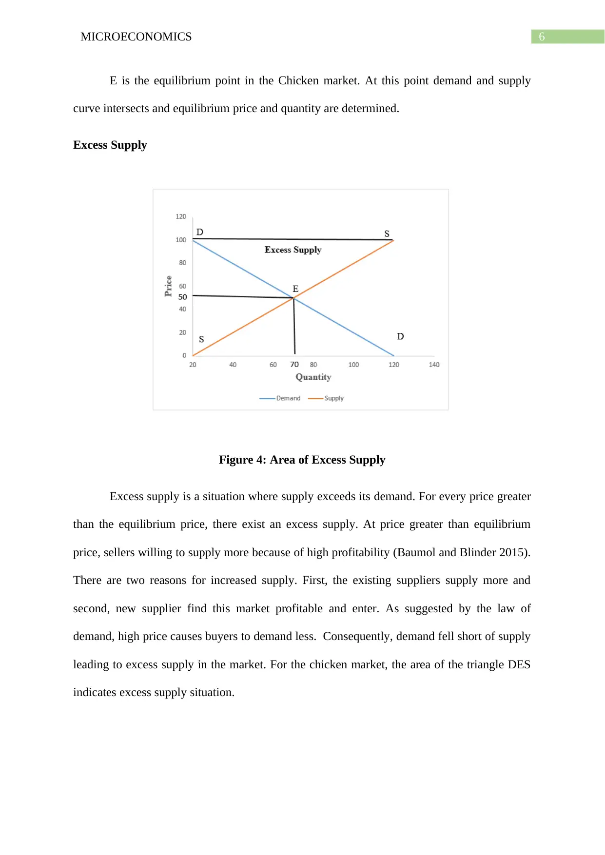
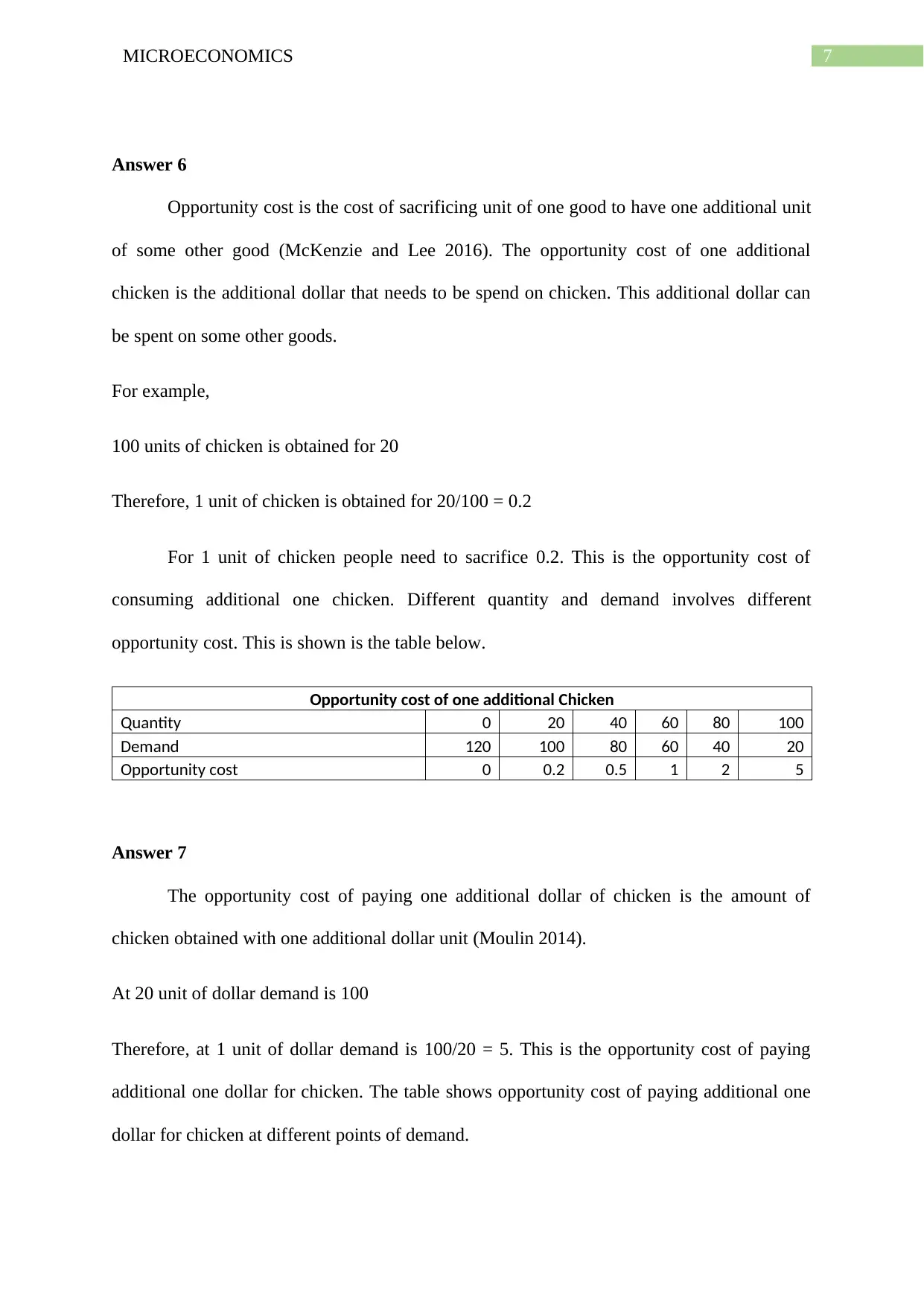
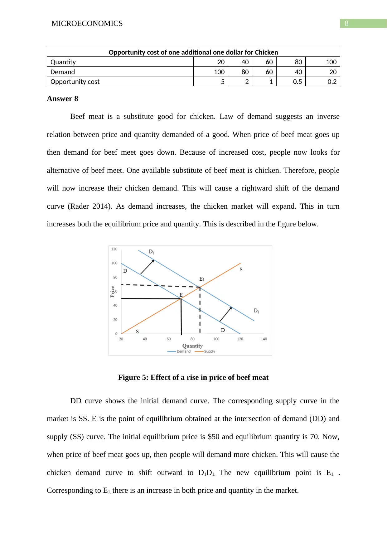
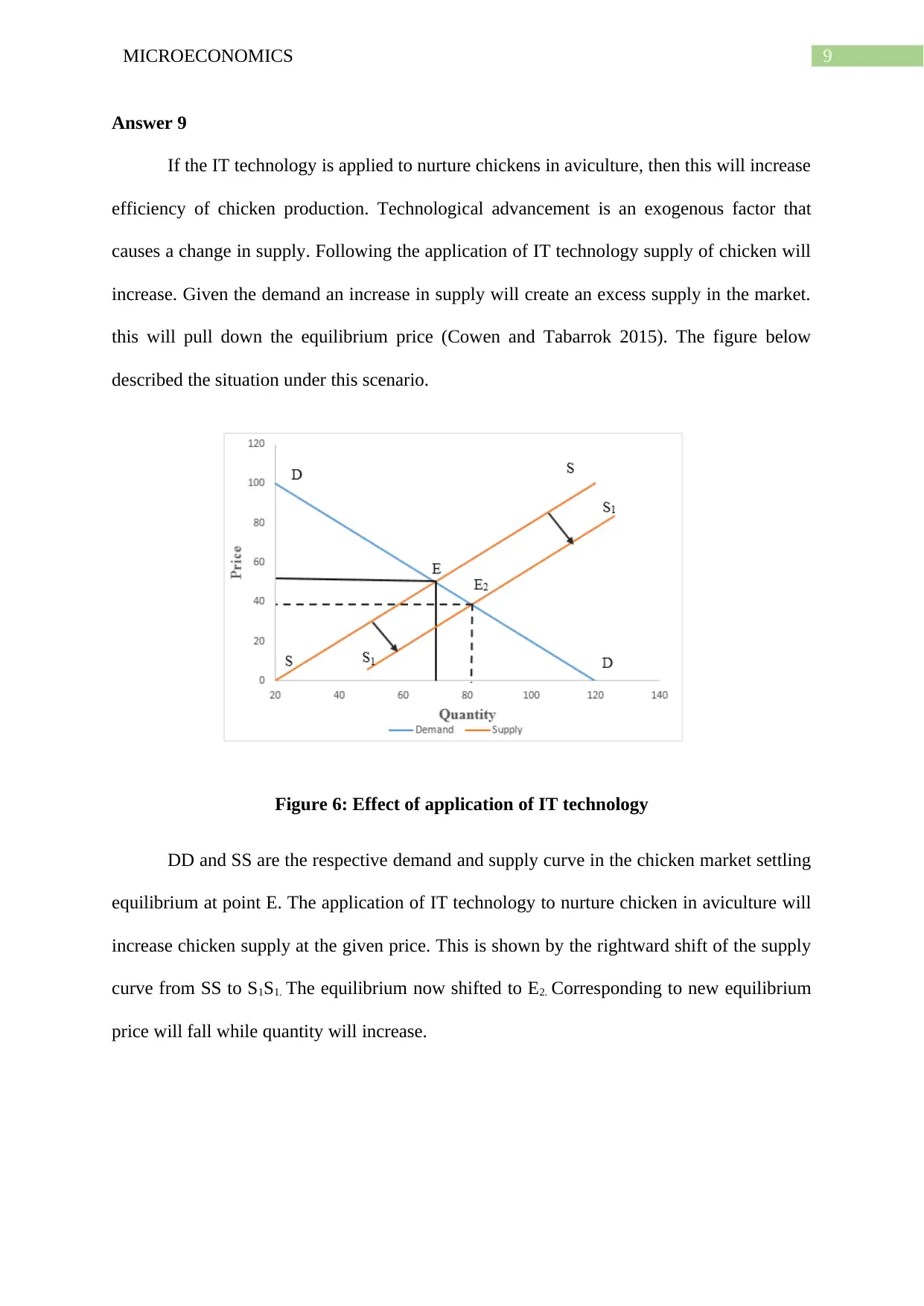
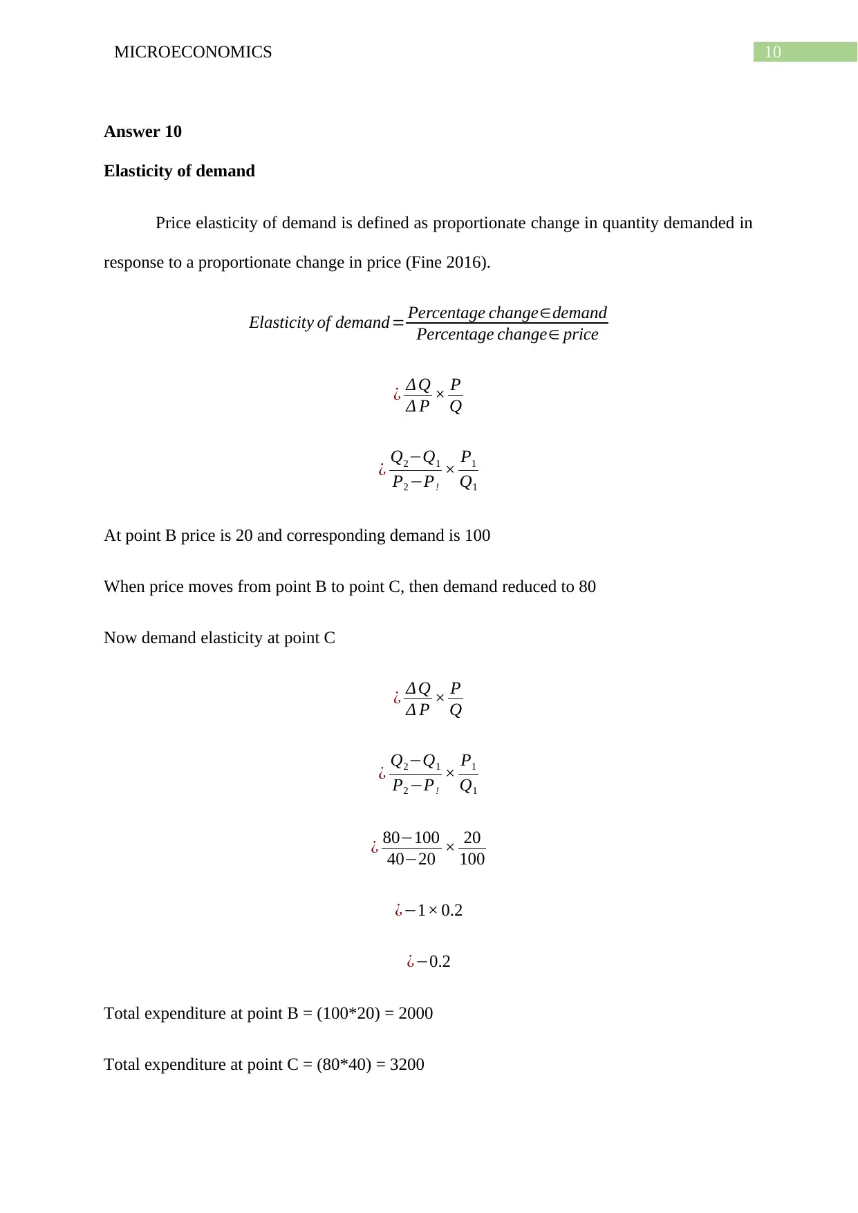
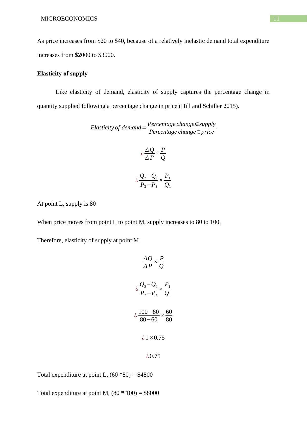
This microeconomics assignment provides a comprehensive analysis of the chicken market, covering demand and supply curves, equilibrium determination, and elasticity calculations. The assignment begins by constructing demand and supply curves based on provided data, deriving their respective equations, and identifying the market equilibrium point where demand equals supply. It further explores concepts such as excess supply, opportunity cost, and the impact of external factors like changes in the price of substitute goods (beef) and technological advancements (IT in aviculture) on the market equilibrium. The assignment also delves into elasticity of demand and supply, calculating these at specific points and analyzing their implications for total expenditure. Finally, it examines consumer and producer surplus, quantifying these measures of economic welfare in the chicken market, demonstrating an equal distribution of total surplus between consumers and producers. Desklib offers a wealth of similar solved assignments and past papers to aid students in their studies.


1 out of 16
Related Documents


Your All-in-One AI-Powered Toolkit for Academic Success.
+13062052269
info@desklib.com
Available 24*7 on WhatsApp / Email
![[object Object]](/_next/static/media/star-bottom.7253800d.svg)
Copyright © 2020–2025 A2Z Services. All Rights Reserved. Developed and managed by ZUCOL.