Microeconomics

This document provides answers to questions on microeconomics, including the concept of profit maximization, demand curve, price elasticity, and the ranking of products based on elasticity. It also includes references for further reading.

Running head: Microeconomics
Microeconomics
Name of the Student
Name of the University
Student ID

1Microeconomics
Table of Contents
Answer 1..........................................................................................................................................2
Answer 2..........................................................................................................................................2
Answer 3..........................................................................................................................................6
References........................................................................................................................................7

2Microeconomics
Answer 1
A firm operating in inelastic portion of demand is not maximizing profit because in order
to maximize profit the firm need to increase its output quantity. However, inelastic demand curve
a slight increase in output quantity will reduce the price by much larger amount and as a result
the total revenue of the firm decreases (Schwartz et al. 2019). Therefore, the firm would not be
able maximize its profit by operating at inelastic portion of demand curve. Inelastic demand
curve is not an ideal situation for a profit maximizing firm.
Answer 2
(a)
Demand function given:
Q=400−3 P+ 4 T + 0.6 A
Therefore, at P=0 and other things as given Q is given as
Q=400−(3 ×0)+(4 × 8000)+(0.6 ×10000)
¿ , Q=400−0+ 32000+6000
¿ , Q=384 00
Again, if Q=0 and other things as given then P is given as
Q=400−3 P+(4 × 8000)+(0.6 × 10000)
¿ , 0=38 400−3 P
¿ , 3 P=38 400

3Microeconomics
¿ , P=12800
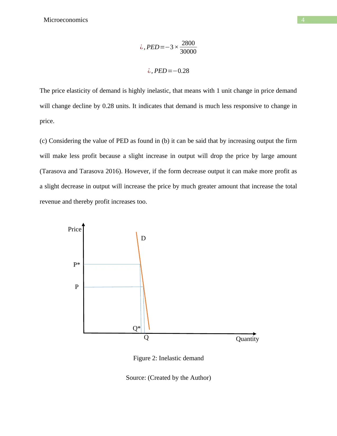
Hence, from the above calculation demand curve can be derived and is given in the diagram
below:
Figure 1: Demand curve
Source: (Created by the Author)
(b)
Current price elasticity of demand considering other factors is given as
Q=400−3 P+ 4 T + 0.6 A
¿ , Q=38 400−3 P
¿ , d Q
dP =−3
¿ , PED=−3 × P
Q
0 5000 10000 15000 20000 25000 30000 35000 40000 45000
0
2000
4000
6000
8000
10000
12000
14000
Demand Curve
Quantity
Price

4Microeconomics
D
Q*
Q
P
P*
Quantity
Price
¿ , PED=−3 × 2800
30000
¿ , PED=−0.28
The price elasticity of demand is highly inelastic, that means with 1 unit change in price demand
will change decline by 0.28 units. It indicates that demand is much less responsive to change in
price.
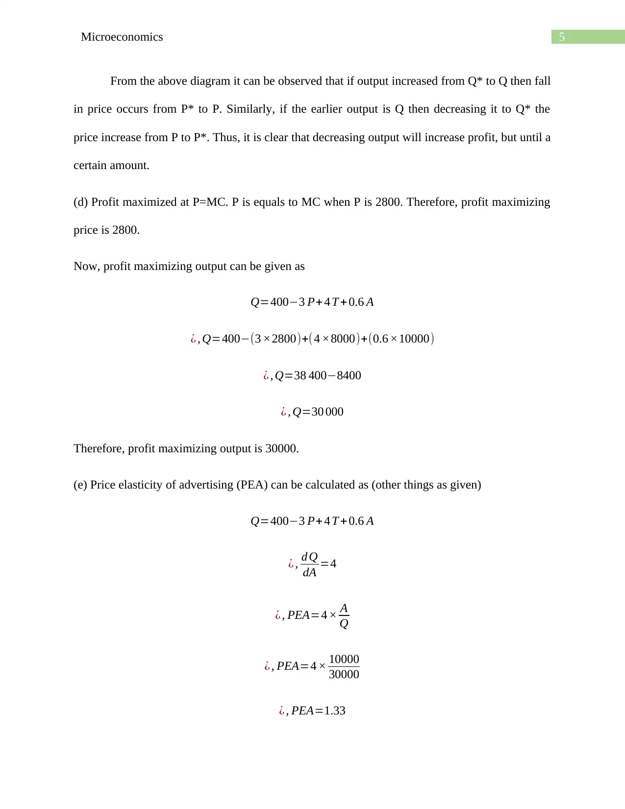
(c) Considering the value of PED as found in (b) it can be said that by increasing output the firm
will make less profit because a slight increase in output will drop the price by large amount
(Tarasova and Tarasova 2016). However, if the form decrease output it can make more profit as
a slight decrease in output will increase the price by much greater amount that increase the total
revenue and thereby profit increases too.
Figure 2: Inelastic demand
Source: (Created by the Author)

5Microeconomics
From the above diagram it can be observed that if output increased from Q* to Q then fall
in price occurs from P* to P. Similarly, if the earlier output is Q then decreasing it to Q* the
price increase from P to P*. Thus, it is clear that decreasing output will increase profit, but until a
certain amount.
(d) Profit maximized at P=MC. P is equals to MC when P is 2800. Therefore, profit maximizing
price is 2800.
Now, profit maximizing output can be given as
Q=400−3 P+ 4 T + 0.6 A
¿ , Q=400−(3 ×2800)+(4 ×8000)+(0.6 ×10000)
¿ , Q=38 400−8400
¿ , Q=30 000
Therefore, profit maximizing output is 30000.
(e) Price elasticity of advertising (PEA) can be calculated as (other things as given)
Q=400−3 P+ 4 T + 0.6 A
¿ , d Q
dA =4
¿ , PEA=4 × A
Q
¿ , PEA=4 × 10000
30000
¿ , PEA=1.33

6Microeconomics
From the value of PEA it can be interpreted that with 1 percent increase in advertising
expenditure sales will increase by 1.33 percent. Thus, to increase sale by 10 percent advertising
expenditure should increase by
Required percenatge increase∈adverytising expenditure= 10
1.33
¿ , Required percenatge increase∈adverytising expenditure=7.52% (appox .)
Answer 3
The list of 3 products is shared below according to descending order of elasticity:
1. Car – Luxury good- most elastic
2. Garments - Normal good- moderately elastic
3. Food – Necessary good – inelastic
Car is a luxury product and is neither used daily nor is a product without which living is
impossible. Thus for such goods people tend to refrain from buying if the price increase by
slightest of amount.
On the other hand, Garment is one of the basic need of life and is required in daily life. However,
it is not required in abundant and thus not essential enough such that one need to buy it regularly.
Thus, change in in it price refrain people from buying it, however price elasticity of demand is
lower than in the case of car (Tarantilis et al. 2015). Furthermore, food is a necessary product
because it is one of the most essential product required to lead life and without food a person will
die of hunger and malnutrition (Hoyos and Artabe 2017). Thus, whatever be the price people
would not reduce their consumption of food. Hence, it the least elastic product in this list.
Therefore, it is justified that why car is ranked at 1, garments at 2 and food at 3.

7Microeconomics
References
Hoyos, D. and Artabe, A., 2017. Regional differences in the price elasticity of residential water
demand in Spain. Water Resources Management, 31(3), pp.847-865.
Schwartz, L.P., Roma, P.G., Henningfield, J.E., Hursh, S.R., Cone, E.J., Buchhalter, A.R., Fant,
R.V. and Schnoll, S.H., 2019. Behavioral economic demand metrics for abuse deterrent and
abuse potential quantification. Drug and alcohol dependence, 198, pp.13-20.
Tarantilis, F., Athanasakis, K., Zavras, D., Vozikis, A. and Kyriopoulos, I., 2015. Estimates of
price and income elasticity in Greece. Greek debt crisis transforming cigarettes into a luxury
good: an econometric approach. BMJ open, 5(1), p.e004748.
Tarasova, V.V. and Tarasov, V.E., 2016. Elasticity for economic processes with memory:
Fractional differential calculus approach. Fractional Differential Calculus, 6(2), pp.219-232.