Microeconomics

This document provides study material and solved assignments for Microeconomics. It covers topics such as negative externality, price ceiling, monopoly, and more. The content includes figures and explanations to help understand the concepts better.

Running head: MICROECONOMICS
Microeconomics
Name of the Student
Name of the University
Author Note

1MICROECONOMICS
Table of Contents
Answer 1....................................................................................................................................2
Answer 2....................................................................................................................................3
Answer 3....................................................................................................................................5
Answer 4....................................................................................................................................6
Answer 5....................................................................................................................................8
Answer 6..................................................................................................................................10
References................................................................................................................................13

2MICROECONOMICS
Answer 1
Figure 1: Negative
externality
Source: (Created by the Author)
In figure 1, the equilibrium of Malaysian garlic market is given by the equilibrium
price $5 and quantity Q1 that occurs at the intersection point between marginal private cost
(MPC) and marginal private benefit (MPB) curve. However, at the quantity there is negative
externality causing from bad breath that created a marginal social cost (MSC), the curve
related to it is shown in the figure. The negative externality generated a social cost in the
form of deadweight loss shown as yellow triangle in the above figure (Demir et al., 2015).
The social cost is equivalent to $2. In the figure, it can be seen that at quantity Q2 where the
price is $7 the deadweight loss can be removed as the price difference is $2 which is
equivalent to the social cost $2. Hence, at this point the consumer surplus decreases and price

3MICROECONOMICS
is higher than the free market (Song, Brown & Glantz, 2014). Thus, this equilibrium is not a
perfectly competitive one.
Devangi suggests that by taxing $2 per kilogram on garlic to maximize social surplus.
From the discussion in the above paragraphs, it can be understood that by taxing the price of
garlic increases to $7 and that will decrease the demand and shifts the MPC curve to left and
the equilibrium price and quantity is $7 and Q2 respectively (Pearce, 2014). Under this tax
policy there will be no deadweight loss as it was in perfectly competitive equilibrium, thus
social gain is higher under $2 tax policy.
Answer 2
Figure 2: Oat
Market
Source: (Created by the Author)
The findings by scientists regarding consumption of oats is a positive as everyone
wants skin glowing skin and healthy hair. This will increase the consumption of oat and thus

4MICROECONOMICS
demand for oat will increase. Simultaneously, increase in wage will increase the cost of
production of oats and thus supply will decrease. Both the cases will affect the price of oat to
increase doubly. The mechanism is explained in figure 2. The initial equilibrium of the oat
market is given by green dot in the figure where price and quantity was P1 and Q1
respectively. After the revelation by scientist regarding the health benefits, the demand for
oat will increase causing demand curve to shift rightward at D2. Hence, perceiving the
demand the oat farmers intend to increase the supply to Q2. This would have been the
equilibrium condition (shown as red dot) with price P2 and quantity Q2, but increase in wage
increased the cost of production for oat farmers and forced them to decrease supply, thus
supply curve will shift leftward to S2 (Panda et al. 2015). Therefore, oat farmers will not
increase the supply as intended and keep on supply Q1. The new equilibrium is at blue dot as
shown in the figure. The price will rise to P3 at the given quantity Q1. Hence, due to
scientific revelation and wage rise, equilibrium price of oat will rise but there will be no
change in equilibrium quantity.
From figure 2 it can be seen that at initial equilibrium price P1 and quantity Q1 the
revenue earned by the oat farmers was given by the orange shaded region. However, after the
revelation of health benefits and increase in cost of labours, the new equilibrium price is P3
and quantity is Q1. At this equilibrium, the revenue earned by the oat farmers is given by the
yellow and orange shaded region. Thus, the total revenue of the farmers increased by the
yellow shaded region in the figure.

5MICROECONOMICS
Answer 3
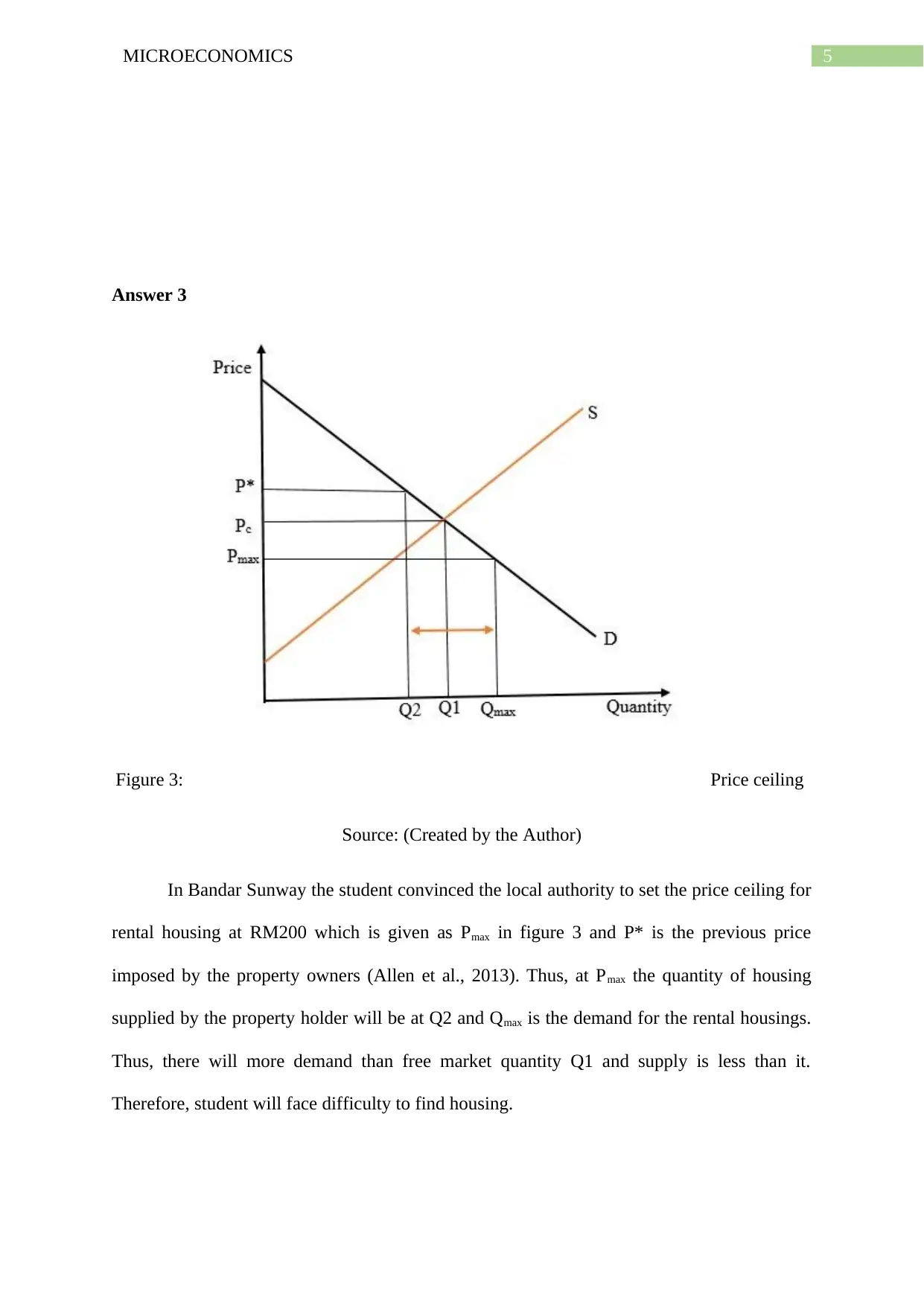
Figure 3: Price ceiling
Source: (Created by the Author)
In Bandar Sunway the student convinced the local authority to set the price ceiling for
rental housing at RM200 which is given as Pmax in figure 3 and P* is the previous price
imposed by the property owners (Allen et al., 2013). Thus, at Pmax the quantity of housing
supplied by the property holder will be at Q2 and Qmax is the demand for the rental housings.
Thus, there will more demand than free market quantity Q1 and supply is less than it.
Therefore, student will face difficulty to find housing.

6MICROECONOMICS
Figure 4:
Price ceiling
Source: (Created by the Author)
After price ceiling, consumer surplus will increase compare to free market
equilibrium shown as blue shaded region in the above diagram and producer surplus will
decrease but there will be dead weight loss show as yellow shaded triangle region (Jacobsen,
2013). However, there is a total surplus loss in the form of deadweight loss.
There will be no incentive for property holders to maintain their quality of rental housing.
However, there will be no such discrimination on gender but possibility of racial
discrimination as there will be very less number of housing available.

7MICROECONOMICS
Answer 4
(a)
(i) Amy’ s accounting profit =Total monetary revenue−Total costs
¿ , Amy ’ s accounting profit =$ ( 3500−1250 )
¿ , Am y' saccounting profit =$ 2250
Am y' s economic profit=Totalmonetary revenue− ( Explicit cost + Implicit cost )
¿ , Am y' s economic profit=$ 3500− ( $ 1250+ $ 2500 )
¿ , Am y' seconomic profit=$ 3500−$ 3750
¿ , Am y' s economic profit=−$ 250
(ii) The economic profit of Amy found to be -$250. Hence, by taking the photo development
job Amy made of loss. However, if Amy had taken the photography job then she would have
made $250 economic profit. Hence, the decision of Amy’s taking the photo development job
was not wise.
(b) Total cost of Ahmad is $220 per day out of which fixed cost is $40. Therefore,
Variable cost =$ (220−40 )
¿ , Variable cost=$ 180
Total revenue earned by Ahmed per day is
Totalrevenue=$ ( 20 ×10 )
¿ , Total revenue=$ 200

8MICROECONOMICS
(i) Now if Ahmad shuts down then the loss generated will be $40 per day which is
the fixed cost
(ii) If Ahmad does not shutdown then the profit or loss generated per day will be
Total profit∨loss=Total revenue−Total cost
¿ , Total profit∨loss=$ ( 200−220 )
¿ , Totalloss=$ 20
(iii) The above findings show that in short run that Ahmad is at least covering its entire
variable cost and contributing towards fixed cost (Pindyck & Rubinfeld, 2014).
Thus, Ahmad will continue to operate in the market in hope of long run profit
(iv) In long run if the same condition exists for Ahmad, then it is better to exit the
market as making loss is not the objective and in a perfectly competitive market,
there are no barriers to exit (Dunne, 2013). Thus, Ahmad exit the market in long
run.
Answer 5

9MICROECONOMICS
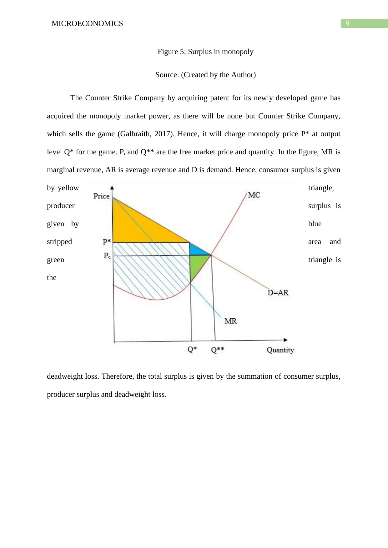
Figure 5: Surplus in monopoly
Source: (Created by the Author)
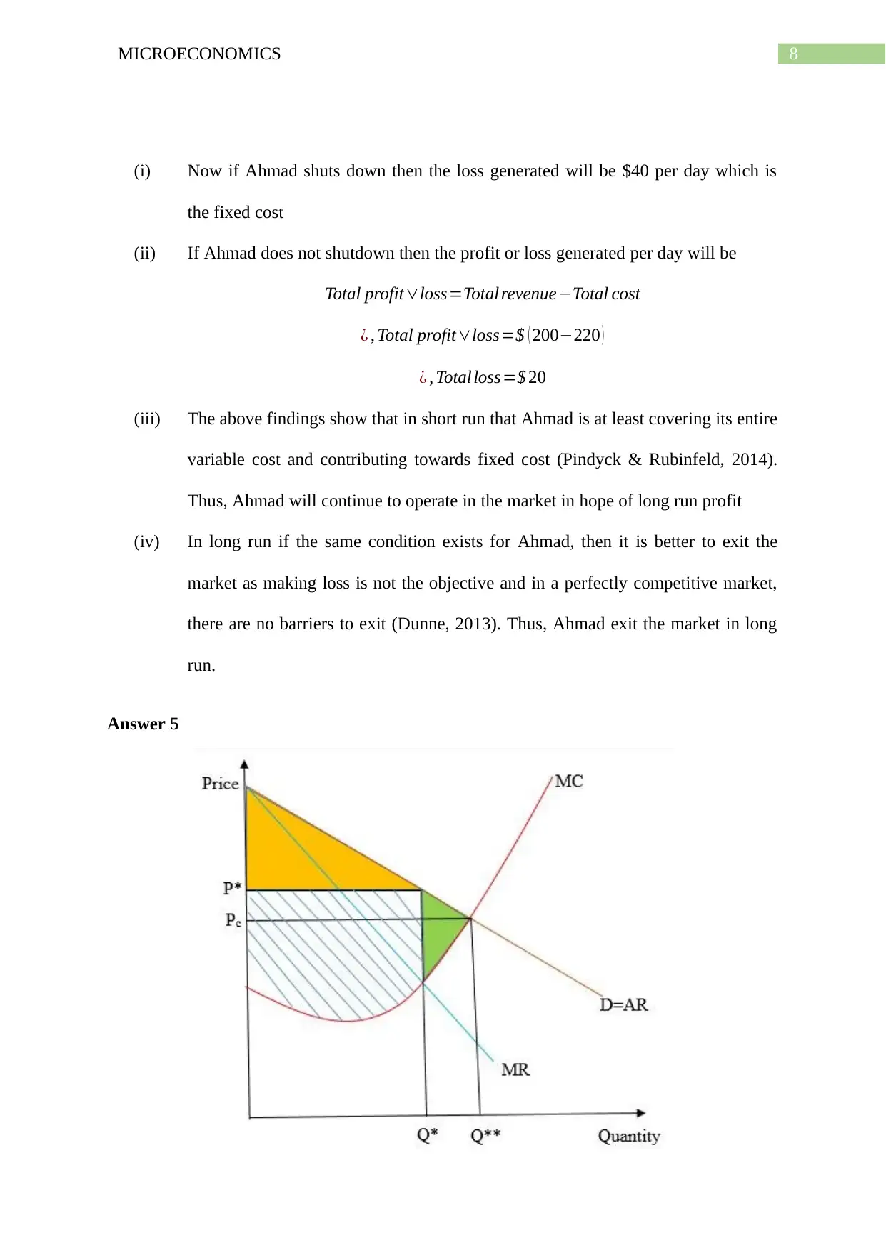
The Counter Strike Company by acquiring patent for its newly developed game has
acquired the monopoly market power, as there will be none but Counter Strike Company,
which sells the game (Galbraith, 2017). Hence, it will charge monopoly price P* at output
level Q* for the game. Pc and Q** are the free market price and quantity. In the figure, MR is
marginal revenue, AR is average revenue and D is demand. Hence, consumer surplus is given
by yellow triangle,
producer surplus is
given by blue
stripped area and
green triangle is
the
deadweight loss. Therefore, the total surplus is given by the summation of consumer surplus,
producer surplus and deadweight loss.

10MICROECONOMICS
Figure 6: Perfect price discrimination
Source: (Created by the Author)
Perfect price discrimination will enable the Counter Strike Company to charge the
price that the customer is willing to pay (Liu & Serfes, 2013). Therefore, the company will
not decide its quantity by the marginal revenue curve rather it will make output decision by
considering marginal cost and demand curve because the incremental revenue gained by the
firm is given by demand curve. No alteration in cost structure will occur in this case.
However, Counter Strike Company will produce as long as the demand is more than marginal
cost, that is until Q** as given in the above figure. Therefore, any extra profit earned by the
company by selling of any incremental unit is given by the difference between marginal cost
and demand curve. Hence, a part of deadweight loss will be recovered and is added in
producer surplus. After, perfect price discrimination there will be no change in consumer
surplus, but a reduction in deadweight loss and is equals the amount of increment in producer
surplus. This increase in producer surplus is given by blue triangle in the above figure.
Although, there will be no change in total surplus
Answer 6
(a)

11MICROECONOMICS
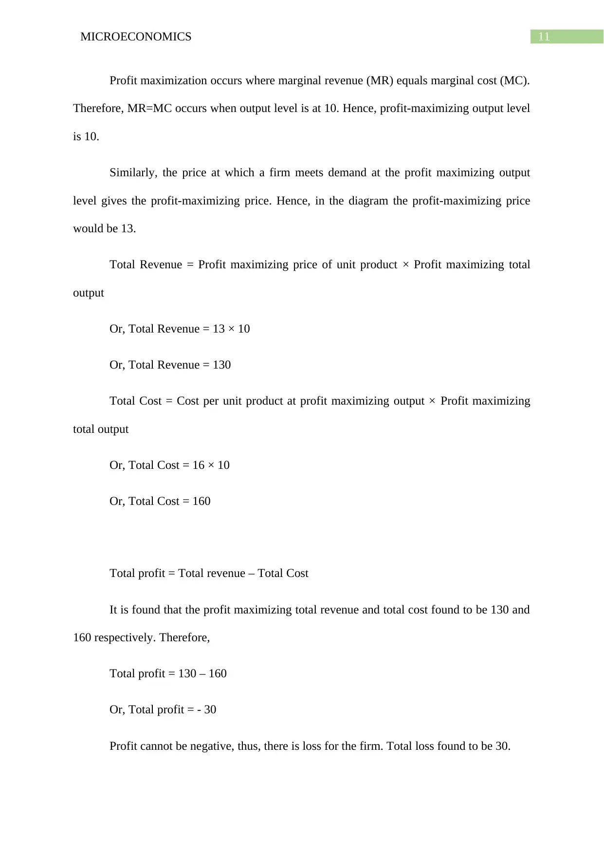
Profit maximization occurs where marginal revenue (MR) equals marginal cost (MC).
Therefore, MR=MC occurs when output level is at 10. Hence, profit-maximizing output level
is 10.
Similarly, the price at which a firm meets demand at the profit maximizing output
level gives the profit-maximizing price. Hence, in the diagram the profit-maximizing price
would be 13.
Total Revenue = Profit maximizing price of unit product × Profit maximizing total
output
Or, Total Revenue = 13 × 10
Or, Total Revenue = 130
Total Cost = Cost per unit product at profit maximizing output × Profit maximizing
total output
Or, Total Cost = 16 × 10
Or, Total Cost = 160
Total profit = Total revenue – Total Cost
It is found that the profit maximizing total revenue and total cost found to be 130 and
160 respectively. Therefore,
Total profit = 130 – 160
Or, Total profit = - 30
Profit cannot be negative, thus, there is loss for the firm. Total loss found to be 30.

12MICROECONOMICS
Figure 7:
Long run Monopolistic competition
Source: (Created by the Author)
In short run, firm in monopolistic competition remain in market and operates as long
as the firm covers its average variable cost, but in the long run under the market condition
shown in the above figure the firms will shut down as there will be loss and in long run no
run operates under loss in any market structure.

13MICROECONOMICS
References
Allen, W. B., Doherty, N. A., Weigelt, K., & Mansfield, E. (2013). Managerial economics:
Theory, applications, and cases. New York: WW Norton.
Demir, E., Huang, Y., Scholts, S., & Van Woensel, T. (2015). A selected review on the
negative externalities of the freight transportation: Modeling and
pricing. Transportation research part E: Logistics and transportation review, 77, 95-
114.
Dunne, T., Klimek, S. D., Roberts, M. J., & Xu, D. Y. (2013). Entry, exit, and the
determinants of market structure. The RAND Journal of Economics, 44(3), 462-487.
Galbraith, J. (2017). American capitalism: The concept of countervailing power. Routledge.
Jacobsen, M. R. (2013). Evaluating US fuel economy standards in a model with producer and
household heterogeneity. American Economic Journal: Economic Policy, 5(2), 148-
87.
Liu, Q., & Serfes, K. (2013). Price discrimination in two‐sided markets. Journal of
Economics & Management Strategy, 22(4), 768-786.
Panda, S., Modak, N. M., Sana, S. S., & Basu, M. (2015). Pricing and replenishment policies
in dual-channel supply chain under continuous unit cost decrease. Applied
Mathematics and Computation, 256, 913-929.
Pearce, D. W. (2014). The Valuation of Social Cost (Routledge Revivals). Routledge.
Pindyck, R., & Rubinfeld, D. (2014). Microeconomics GE. Pearson Australia Pty Limited.

14MICROECONOMICS
Song, A. V., Brown, P., & Glantz, S. A. (2014). When health policy and empirical evidence
collide: the case of cigarette package warning labels and economic consumer
surplus. American journal of public health, 104(2), e42-e51.