Microeconomics Assignment: Analysis of Market Dynamics and Policies
VerifiedAdded on 2020/05/28
|13
|1900
|412
Homework Assignment
AI Summary
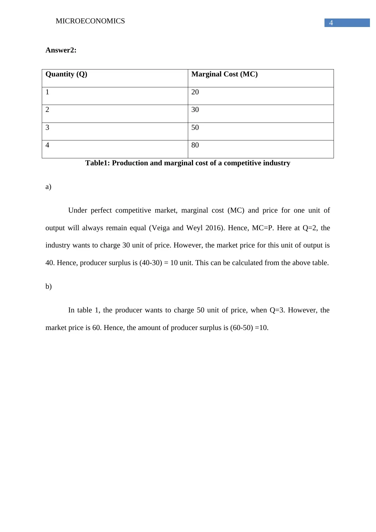
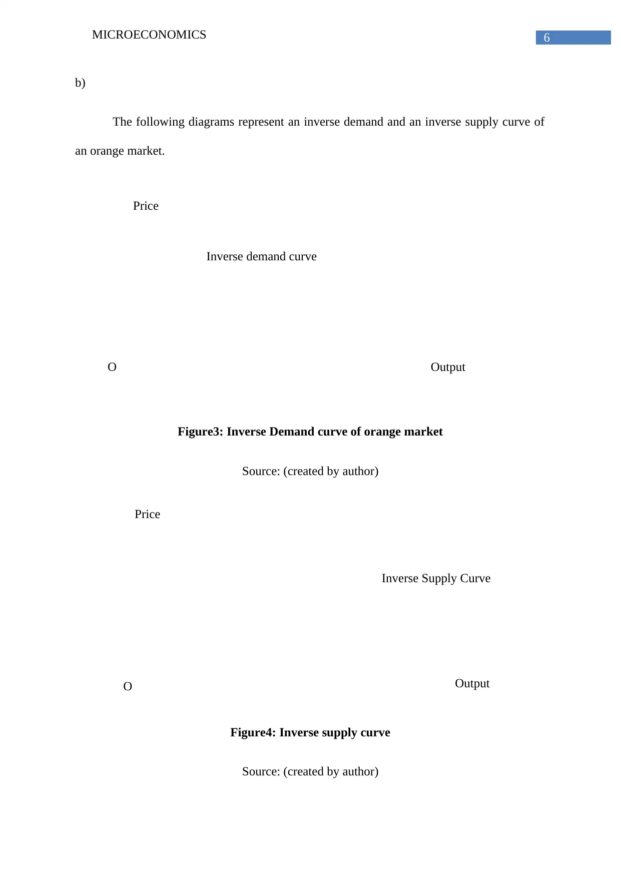
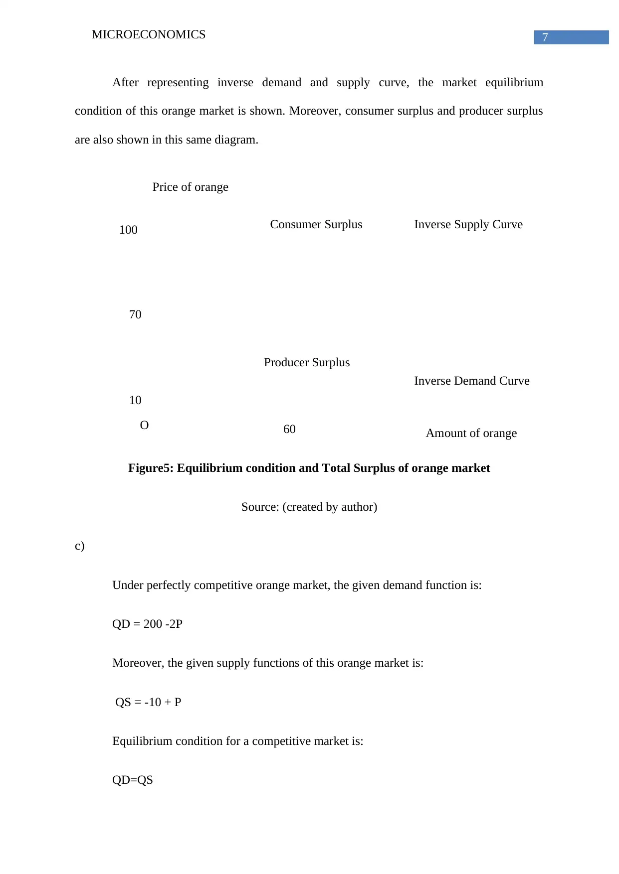
This microeconomics assignment delves into various aspects of market analysis and economic policies. The solution begins by examining the effects of export subsidies and import quotas on the Australian and Canadian beef markets, analyzing changes in consumer and producer surplus, and the impact on government revenue. It then explores the principles of a competitive industry, calculating producer surplus based on marginal costs and market prices. The assignment further investigates inverse demand and supply curves, determining market equilibrium, and calculating consumer and producer surplus in the orange market. Finally, it addresses the consequences of taxes on Alcopops, considering the emergence of black markets and evaluating the effectiveness of such policies. The solution integrates graphical representations and economic principles to provide a comprehensive understanding of the topics covered.

1 out of 13
Related Documents


Your All-in-One AI-Powered Toolkit for Academic Success.
+13062052269
info@desklib.com
Available 24*7 on WhatsApp / Email
![[object Object]](/_next/static/media/star-bottom.7253800d.svg)
Copyright © 2020–2026 A2Z Services. All Rights Reserved. Developed and managed by ZUCOL.