Investigating Milling Process Parameters via ANSYS Simulation
VerifiedAdded on 2023/03/31
|20
|3817
|287
Report
AI Summary
This report details a methodology for analyzing milling process parameters using ANSYS simulation and SolidWorks software. The study focuses on the impact of material properties on tool life and surface finish, simulating a titanium alloy cutting tool with aluminum and stainless steel workpieces. The ANSYS Explicit Dynamics module is employed, outlining steps from analysis system creation to post-processing, including defining engineering data, geometry, part behavior, connections, symmetry, remote points, meshing, analysis settings, initial conditions, and load application. The results section presents Von-Mises stress, elastic strain, and total deformation for both material combinations. Key factors affecting cutting tool life are discussed, such as cutting speed, workpiece physical properties, area of cut, feed-to-depth ratio, tool shape, lubricant effect, and cutting nature. The report concludes with a summary of findings and recommendations to improve tool life, emphasizing the importance of optimized parameters for enhanced milling process efficiency. Desklib provides students access to this and many more solved assignments.

Milling process parameters
ANSYS SIMULATION OF MILLING TOOL
ANSYS SIMULATION OF MILLING TOOL
Paraphrase This Document
Need a fresh take? Get an instant paraphrase of this document with our AI Paraphraser
Table of Contents
1. Methodology............................................................................................................................2
1.1 ANSYS Steps....................................................................................................................2
1.2 Major factors affecting the cutting tool life......................................................................8
1.2.1 Cutting Speed.............................................................................................................8
1.2.2 Physical Properties of Work Piece............................................................................8
1.2.3 Area of Cut................................................................................................................9
1.2.4 Ratio of Feed to Depth of Cut....................................................................................9
1.2.5 Shape and Angles of Tools......................................................................................10
1.2.6 Effect of Lubricant...................................................................................................10
1.2.7 Nature of Cutting.....................................................................................................10
2. ANSYS results.......................................................................................................................12
2.1 Aluminum work piece vs Titanium alloy cutting tool....................................................12
2.1.1 Von-Mises Stress.....................................................................................................12
2.1.2 Elastic Strain............................................................................................................12
2.1.3 Total Deformation...................................................................................................13
2.2 Stainless steel work piece vs Titanium alloy cutting tool...............................................13
2.2.1 Von-mises Stress.....................................................................................................13
2.2.2 Elastic Strain............................................................................................................14
2.2.3 Total Deformation...................................................................................................14
3. Summary of Findings.............................................................................................................15
4. Recommendations for improve tool life.................................................................................15
5. References..............................................................................................................................17
1
1. Methodology
In this section of the methodology used for the analysis is explained. Here ANSYS 19.0 software
and Solid works software are used for the simulation and designing. Tool life and surface finish
of the product produced by the milling process mainly depends on the milling process
parameters. In general, there are a different set of milling parameters are there. Among them,
material properties are focused on this research. Here two different work materials and titanium
alloy cutting tool are simulated.
Cutting tool material is selected as titanium and its mechanical properties are given below.
Tensile Strength 220 MPa
Modulus of elasticity 116 GPa
Shear Modulus 43 GPa
Hardness Number 70 BHN
Density 4.50 g/cc
Melting Point 1670 C
Poisson Ratio 0.34
Thermal Conductivity 17 W/mK
Work Piece Material
Aluminum
Structured Steel
1.1 ANSYS Steps
Explicit dynamics is a simulation model that included the applied loads and interactions, setting
up the model, and solving the model in the nonlinear dynamic responsive method. The workflow
of the explicit dynamics is given in the following steps (An et al., 2014).
The first step is the creation of the analysis system. For creating the analysis, from the toolbox,
we need to expand the standard analysis folder. Then drag the template onto project schematic.
2
⊘ This is a preview!⊘
Do you want full access?
Subscribe today to unlock all pages.
Trusted by 1+ million students worldwide
In the analysis system consist of an array of cells, they are displayed in the vertical form and
each cell is denoted as a component of the system. To indicate every cell in the system need to
right-click the cell and choose the edit option. The explicit dynamic solver is a type of double
precision. The explicit dynamics support the ms, mm, and mg solver unit system. (Baron and
Rolland, 2015)
The second step is defining the engineering data. In this part, the properties of the material are
described. Based on the application the material properties are varied. The material properties
can be temperature dependent, nonlinear or linear. The nonlinear material, hyper elastic material,
and plasticity materials properties are present in the tabular format. The linear materials have
constant properties. If we use the material for the dynamic analysis means it must contain the
density. For each analysis, we have defined the material properties. Using the Engineer Data tab
we add materials to the material library. To perform any operations on materials, right-click the
Engineering Data tab and click the edit option.
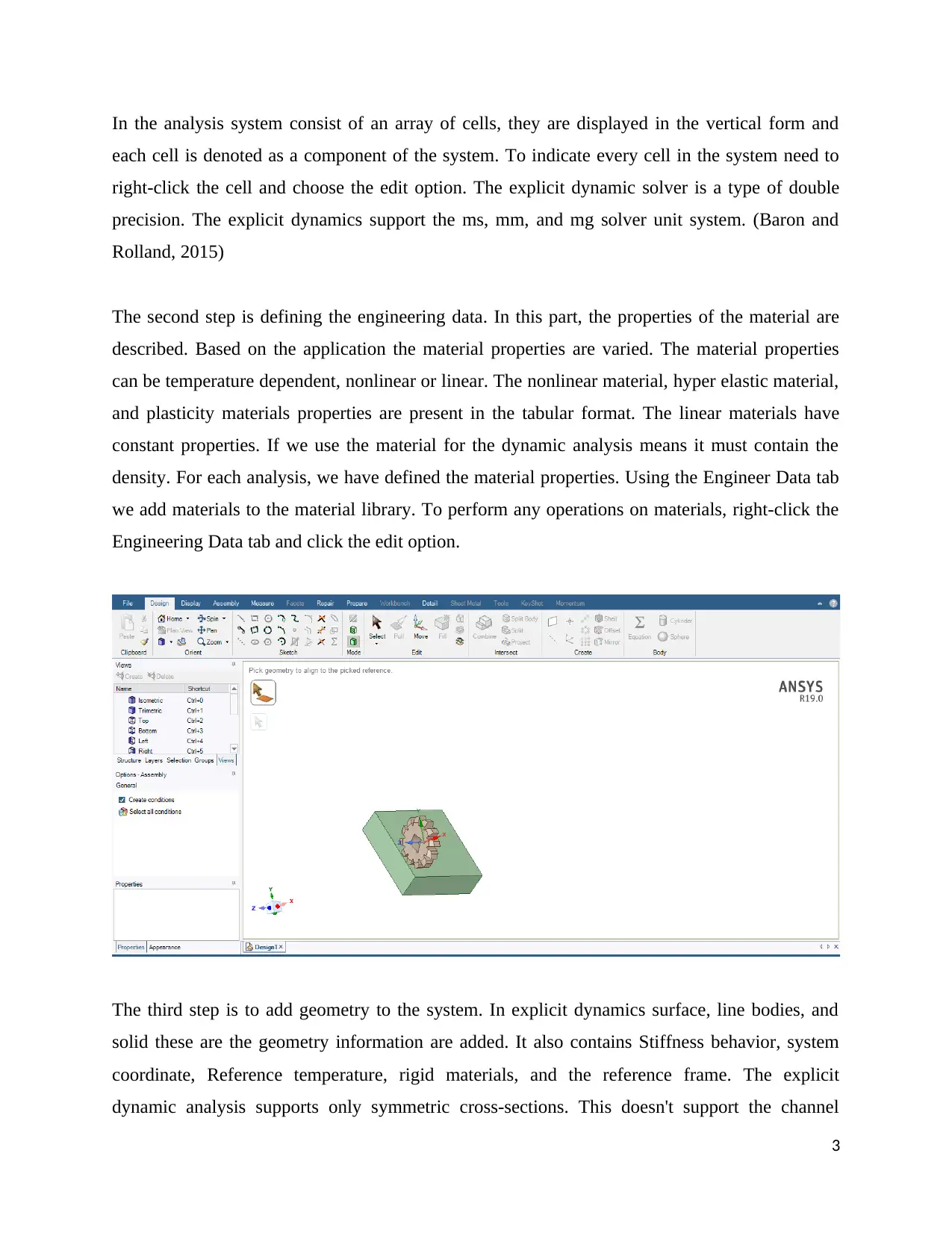
The third step is to add geometry to the system. In explicit dynamics surface, line bodies, and
solid these are the geometry information are added. It also contains Stiffness behavior, system
coordinate, Reference temperature, rigid materials, and the reference frame. The explicit
dynamic analysis supports only symmetric cross-sections. This doesn't support the channel
3
each cell is denoted as a component of the system. To indicate every cell in the system need to
right-click the cell and choose the edit option. The explicit dynamic solver is a type of double
precision. The explicit dynamics support the ms, mm, and mg solver unit system. (Baron and
Rolland, 2015)
The second step is defining the engineering data. In this part, the properties of the material are
described. Based on the application the material properties are varied. The material properties
can be temperature dependent, nonlinear or linear. The nonlinear material, hyper elastic material,
and plasticity materials properties are present in the tabular format. The linear materials have
constant properties. If we use the material for the dynamic analysis means it must contain the
density. For each analysis, we have defined the material properties. Using the Engineer Data tab
we add materials to the material library. To perform any operations on materials, right-click the
Engineering Data tab and click the edit option.
The third step is to add geometry to the system. In explicit dynamics surface, line bodies, and
solid these are the geometry information are added. It also contains Stiffness behavior, system
coordinate, Reference temperature, rigid materials, and the reference frame. The explicit
dynamic analysis supports only symmetric cross-sections. This doesn't support the channel
3
Paraphrase This Document
Need a fresh take? Get an instant paraphrase of this document with our AI Paraphraser
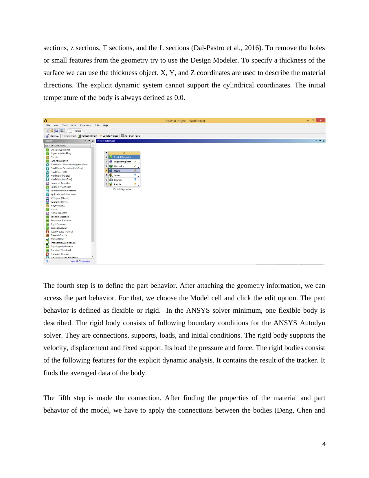
sections, z sections, T sections, and the L sections (Dal-Pastro et al., 2016). To remove the holes
or small features from the geometry try to use the Design Modeler. To specify a thickness of the
surface we can use the thickness object. X, Y, and Z coordinates are used to describe the material
directions. The explicit dynamic system cannot support the cylindrical coordinates. The initial
temperature of the body is always defined as 0.0.
The fourth step is to define the part behavior. After attaching the geometry information, we can
access the part behavior. For that, we choose the Model cell and click the edit option. The part
behavior is defined as flexible or rigid. In the ANSYS solver minimum, one flexible body is
described. The rigid body consists of following boundary conditions for the ANSYS Autodyn
solver. They are connections, supports, loads, and initial conditions. The rigid body supports the
velocity, displacement and fixed support. Its load the pressure and force. The rigid bodies consist
of the following features for the explicit dynamic analysis. It contains the result of the tracker. It
finds the averaged data of the body.
The fifth step is made the connection. After finding the properties of the material and part
behavior of the model, we have to apply the connections between the bodies (Deng, Chen and
4
Zhou, 2013). There are many connection features are presents. They are springs, beam
connections, joints, end releases, bearings, and mesh connections.
To connect the line body to line body it contains the following constraints.
In body interactions, contact detection must be in proximity based.
In the body interactions, details view the edge to edge connection is set to be yes.
It has a frictional interaction type.
For the explicit dynamic analyses joints, beam, and spring connections are not applicable. It also
doesn't support the contact tool. Using the keyword snippets option contacts between solids and
line bodies are implemented in the explicit dynamics. To join the tetrahedral meshes multipart
are recommended instead of bonds.
The sixth step is setting up symmetry. In this step, the design modeler cut the full model into
small parts and takes only the symmetric part. After that, we need to insert the symmetry model
into the tree. Then it will show the types of regions, symmetry in the mechanical application and
symmetry defined in design modeler options (Djodikusumo, Diasta and Sanjaya Awaluddin,
2016).
The seventh point is defining the remote points. Remote points are used to provide a connection
to a solid model. Multipoint constraint equations are used for connections in the solver. The
remote points are working under the following boundary conditions. They are bearing, joints,
beam connection, point mass, thermal point mass, spring, remote force and moment. If we use a
remote point to multiple remote moments or remote force it will generate a warning message. So
remote point only used for a one moment and one remote force (Effgen and Kirsch, 2013).
The next step is to apply the mesh controls and preview mesh. In this process, the geometry is
divided into nodes and elements. The mesh has the properties of the material in a mathematical
manner. There are several mesh methods are available. They are Hex dominant meshing, patch
dependent shell meshing, swept volume meshing, patch independent tetrahedral meshing, patch
dependent shell meshing, and multimode volume meshing. Mesh controls are used to reduce the
size of the problem. In the explicit dynamics analyses multimode or swept meshes are used
5
⊘ This is a preview!⊘
Do you want full access?
Subscribe today to unlock all pages.
Trusted by 1+ million students worldwide
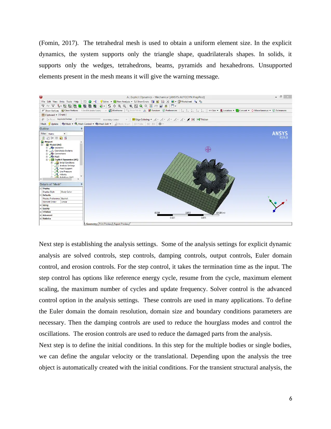
(Fomin, 2017). The tetrahedral mesh is used to obtain a uniform element size. In the explicit
dynamics, the system supports only the triangle shape, quadrilaterals shapes. In solids, it
supports only the wedges, tetrahedrons, beams, pyramids and hexahedrons. Unsupported
elements present in the mesh means it will give the warning message.
Next step is establishing the analysis settings. Some of the analysis settings for explicit dynamic
analysis are solved controls, step controls, damping controls, output controls, Euler domain
control, and erosion controls. For the step control, it takes the termination time as the input. The
step control has options like reference energy cycle, resume from the cycle, maximum element
scaling, the maximum number of cycles and update frequency. Solver control is the advanced
control option in the analysis settings. These controls are used in many applications. To define
the Euler domain the domain resolution, domain size and boundary conditions parameters are
necessary. Then the damping controls are used to reduce the hourglass modes and control the
oscillations. The erosion controls are used to reduce the damaged parts from the analysis.
Next step is to define the initial conditions. In this step for the multiple bodies or single bodies,
we can define the angular velocity or the translational. Depending upon the analysis the tree
object is automatically created with the initial conditions. For the transient structural analysis, the
6
Paraphrase This Document
Need a fresh take? Get an instant paraphrase of this document with our AI Paraphraser
initial condition is used as velocity (Hsiao and Huang, 2014). The Transient state and steady
state analysis use the initial temperature value initial temperature object.
Next is apply for load and support. In this step based on the analysis, the load and supply will be
applied. For example, pressure and force for loads and displacement for supports used as stress
analysis. For the thermal analysis, it uses different load and stress values. The load value is
applied to the transient structural, magnetostatic, thermal-electric, static structural analyses. If
bodies have a reference frame of eulerian load and supports are not valid in those situations (Li
and Yao, 2013).
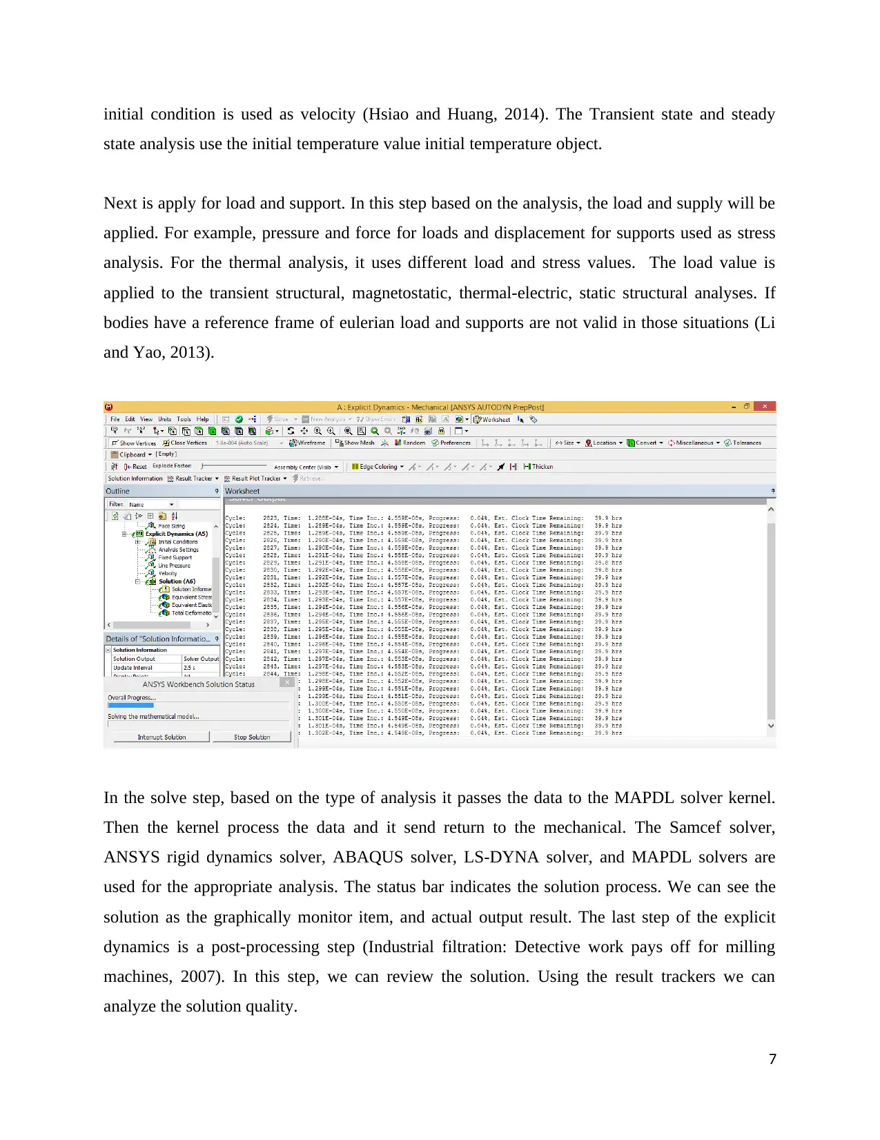
In the solve step, based on the type of analysis it passes the data to the MAPDL solver kernel.
Then the kernel process the data and it send return to the mechanical. The Samcef solver,
ANSYS rigid dynamics solver, ABAQUS solver, LS-DYNA solver, and MAPDL solvers are
used for the appropriate analysis. The status bar indicates the solution process. We can see the
solution as the graphically monitor item, and actual output result. The last step of the explicit
dynamics is a post-processing step (Industrial filtration: Detective work pays off for milling
machines, 2007). In this step, we can review the solution. Using the result trackers we can
analyze the solution quality.
7
state analysis use the initial temperature value initial temperature object.
Next is apply for load and support. In this step based on the analysis, the load and supply will be
applied. For example, pressure and force for loads and displacement for supports used as stress
analysis. For the thermal analysis, it uses different load and stress values. The load value is
applied to the transient structural, magnetostatic, thermal-electric, static structural analyses. If
bodies have a reference frame of eulerian load and supports are not valid in those situations (Li
and Yao, 2013).
In the solve step, based on the type of analysis it passes the data to the MAPDL solver kernel.
Then the kernel process the data and it send return to the mechanical. The Samcef solver,
ANSYS rigid dynamics solver, ABAQUS solver, LS-DYNA solver, and MAPDL solvers are
used for the appropriate analysis. The status bar indicates the solution process. We can see the
solution as the graphically monitor item, and actual output result. The last step of the explicit
dynamics is a post-processing step (Industrial filtration: Detective work pays off for milling
machines, 2007). In this step, we can review the solution. Using the result trackers we can
analyze the solution quality.
7
1.2 Major factors affecting the cutting tool life
1.2.1 Cutting Speed
It has an extreme impact on tool life. A tool’s life is decremented when the fragmentation the
level is incremented. The principle of wear is reliant on fragmentation level due to the major
wear must be border wear or dip wear if the speediness is high. It must be seen that the turning of
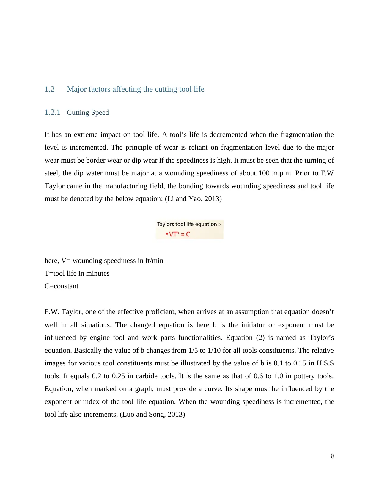
steel, the dip water must be major at a wounding speediness of about 100 m.p.m. Prior to F.W
Taylor came in the manufacturing field, the bonding towards wounding speediness and tool life
must be denoted by the below equation: (Li and Yao, 2013)
here, V= wounding speediness in ft/min
T=tool life in minutes
C=constant
F.W. Taylor, one of the effective proficient, when arrives at an assumption that equation doesn’t
well in all situations. The changed equation is here b is the initiator or exponent must be
influenced by engine tool and work parts functionalities. Equation (2) is named as Taylor’s
equation. Basically the value of b changes from 1/5 to 1/10 for all tools constituents. The relative
images for various tool constituents must be illustrated by the value of b is 0.1 to 0.15 in H.S.S
tools. It equals 0.2 to 0.25 in carbide tools. It is the same as that of 0.6 to 1.0 in pottery tools.
Equation, when marked on a graph, must provide a curve. Its shape must be influenced by the
exponent or index of the tool life equation. When the wounding speediness is incremented, the
tool life also increments. (Luo and Song, 2013)
8
1.2.1 Cutting Speed
It has an extreme impact on tool life. A tool’s life is decremented when the fragmentation the
level is incremented. The principle of wear is reliant on fragmentation level due to the major
wear must be border wear or dip wear if the speediness is high. It must be seen that the turning of
steel, the dip water must be major at a wounding speediness of about 100 m.p.m. Prior to F.W
Taylor came in the manufacturing field, the bonding towards wounding speediness and tool life
must be denoted by the below equation: (Li and Yao, 2013)
here, V= wounding speediness in ft/min
T=tool life in minutes
C=constant
F.W. Taylor, one of the effective proficient, when arrives at an assumption that equation doesn’t
well in all situations. The changed equation is here b is the initiator or exponent must be
influenced by engine tool and work parts functionalities. Equation (2) is named as Taylor’s
equation. Basically the value of b changes from 1/5 to 1/10 for all tools constituents. The relative
images for various tool constituents must be illustrated by the value of b is 0.1 to 0.15 in H.S.S
tools. It equals 0.2 to 0.25 in carbide tools. It is the same as that of 0.6 to 1.0 in pottery tools.
Equation, when marked on a graph, must provide a curve. Its shape must be influenced by the
exponent or index of the tool life equation. When the wounding speediness is incremented, the
tool life also increments. (Luo and Song, 2013)
8
⊘ This is a preview!⊘
Do you want full access?
Subscribe today to unlock all pages.
Trusted by 1+ million students worldwide
1.2.2 Physical Properties of Work Piece
The wounding speediness must be influenced by the work parts and tool constituents. The table
given below represents the relative images for various tool and work parts constituents. It must
be seen that tool life must be connected with the minute structure of a task. Basically hard micro-
particles in the matrix must give pitiable tool life (MA, 2014). Tool life is good with high size of
the grain. It must be seen that the same metal constructions will display the same machine
functionalities. The result of attributes of constituents is denoted by this equation:
HB =Brinell number.
1.2.3 Area of Cut
The wounding speediness v is conversely relative to the point of fragmentation and it is denoted
by this equation:
V is the wounding speediness,
A is the point of fragmentation,
k, b,c are constants.
In equation (3) since V α 1/A.
If the graph is plotted within the wounding speediness and point of fragmentation, it must be
seen that the area increments and the wounding speediness decrements.
1.2.4 The ratio of Feed to Depth of Cut
When there is extra feed, extra local action, and warming of the tool at the chip tool the interface
must happen (Malik, Przytocka and Karpiuk, 2019). For a similar point of fragmentation, if the
distance must increments doubly and the feed must decrement to half, the fragmentation
speediness must be incremented by 40%.It must be seen that the proportion of distance to the
9
Paraphrase This Document
Need a fresh take? Get an instant paraphrase of this document with our AI Paraphraser
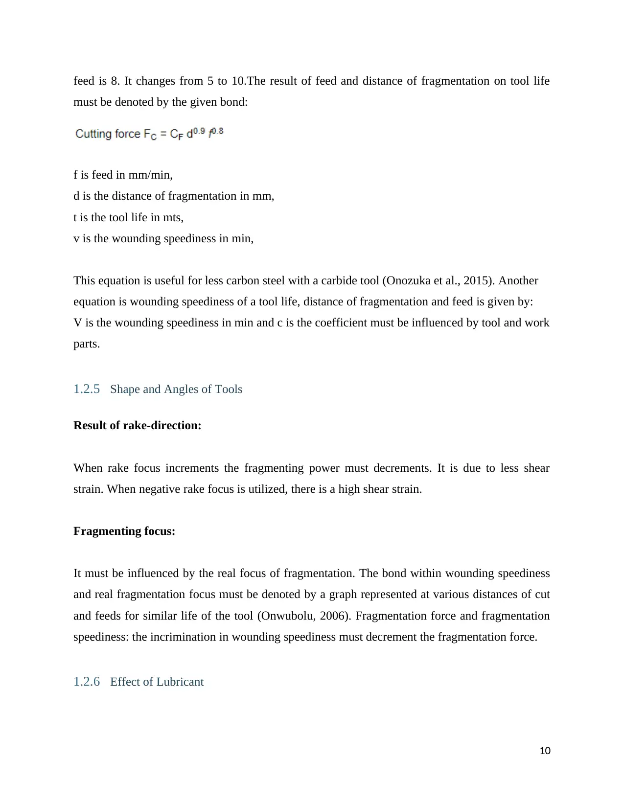
feed is 8. It changes from 5 to 10.The result of feed and distance of fragmentation on tool life
must be denoted by the given bond:
f is feed in mm/min,
d is the distance of fragmentation in mm,
t is the tool life in mts,
v is the wounding speediness in min,
This equation is useful for less carbon steel with a carbide tool (Onozuka et al., 2015). Another
equation is wounding speediness of a tool life, distance of fragmentation and feed is given by:
V is the wounding speediness in min and c is the coefficient must be influenced by tool and work
parts.
1.2.5 Shape and Angles of Tools
Result of rake-direction:
When rake focus increments the fragmenting power must decrements. It is due to less shear
strain. When negative rake focus is utilized, there is a high shear strain.
Fragmenting focus:
It must be influenced by the real focus of fragmentation. The bond within wounding speediness
and real fragmentation focus must be denoted by a graph represented at various distances of cut
and feeds for similar life of the tool (Onwubolu, 2006). Fragmentation force and fragmentation
speediness: the incrimination in wounding speediness must decrement the fragmentation force.
1.2.6 Effect of Lubricant
10

It decrements the fragmentation forces. So tool life automatically increases with the use of
lubrication. Proper lubrication helps to improve the tool life. At the same time, it also has some
negative effects like to the machine (Schlüter, Hübner and de Souza, 2015).
1.2.7 Nature of Cutting
It is dependent on tool life. In comparison with nonstop fragmentation, tool life is very good than
in recurrent fragmentation (Schönemann, Riemer and Brinksmeier, 2016).
r – Nose radius
11
⊘ This is a preview!⊘
Do you want full access?
Subscribe today to unlock all pages.
Trusted by 1+ million students worldwide
1 out of 20
Your All-in-One AI-Powered Toolkit for Academic Success.
+13062052269
info@desklib.com
Available 24*7 on WhatsApp / Email
![[object Object]](/_next/static/media/star-bottom.7253800d.svg)
Unlock your academic potential
Copyright © 2020–2026 A2Z Services. All Rights Reserved. Developed and managed by ZUCOL.