Modelling & Simulation Project: Finite Element Analysis with Abaqus

This project report details a finite element analysis (FEA) of a truss structure and a concrete overpass structure using Abaqus software. The assignment, ENGIN5302, involves modeling the structures, defining material properties, applying loads and boundary conditions, and meshing the models. Task 1 focuses on analyzing a truss bridge under distributed and point loads, including a convergence study to determine the optimal number of elements per member. The results include deformed shapes, stress contours, and the location of maximum stress and deflection. Task 2 analyzes a concrete overpass. The report includes detailed methodology, algorithms, screenshots of results, and discussions on analysis, error estimation, and convergence. The project emphasizes the importance of simulation in engineering design and the use of Abaqus for solving complex structural problems. The report also provides insights into the impact of mesh resolution on the accuracy of the FEA results.

Modeling and simulation
Student name
Institution

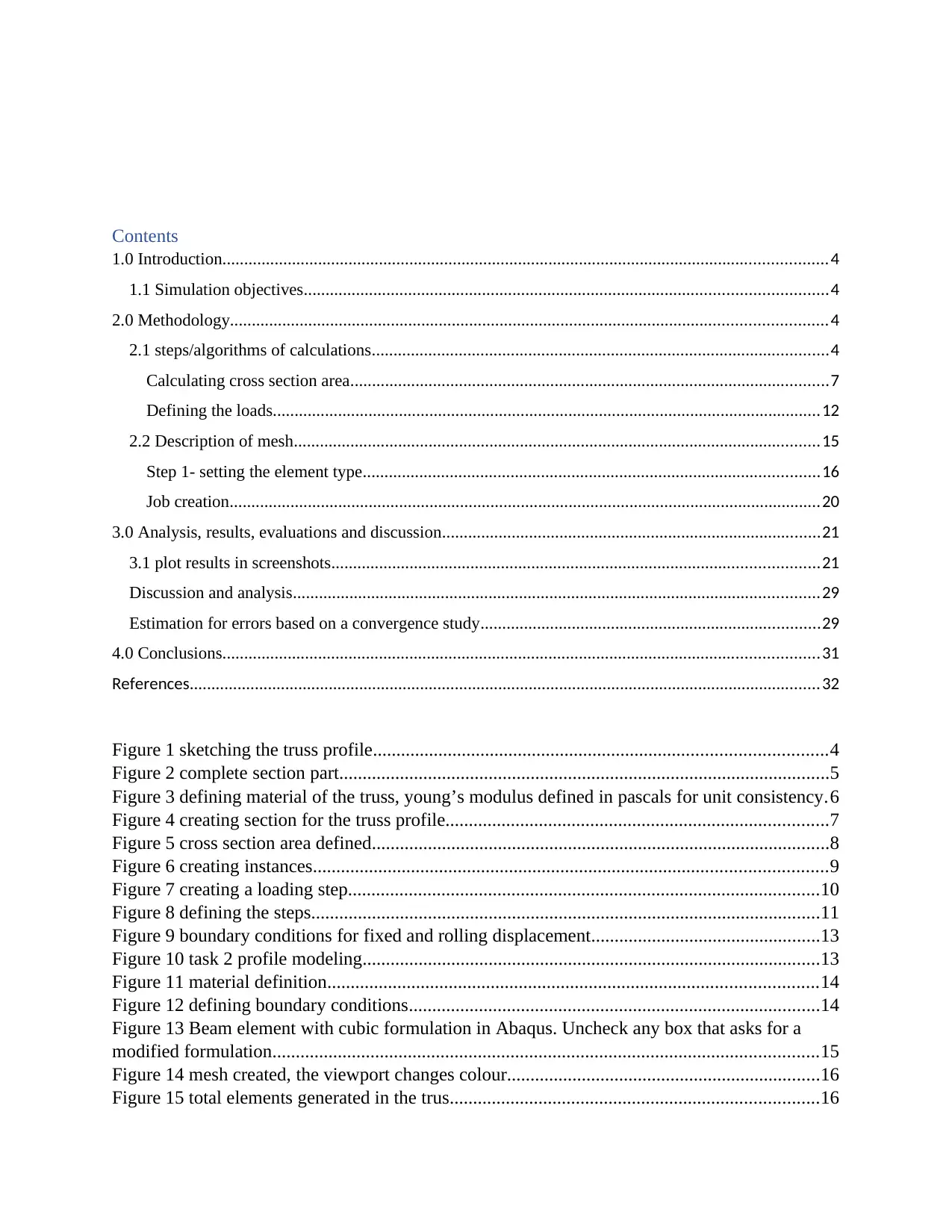
Contents
1.0 Introduction...........................................................................................................................................4
1.1 Simulation objectives........................................................................................................................4
2.0 Methodology.........................................................................................................................................4
2.1 steps/algorithms of calculations.........................................................................................................4
Calculating cross section area..............................................................................................................7
Defining the loads..............................................................................................................................12
2.2 Description of mesh.........................................................................................................................15
Step 1- setting the element type.........................................................................................................16
Job creation........................................................................................................................................20
3.0 Analysis, results, evaluations and discussion.......................................................................................21
3.1 plot results in screenshots................................................................................................................21
Discussion and analysis.........................................................................................................................29
Estimation for errors based on a convergence study..............................................................................29
4.0 Conclusions.........................................................................................................................................31
References.................................................................................................................................................32
Figure 1 sketching the truss profile.................................................................................................4
Figure 2 complete section part.........................................................................................................5
Figure 3 defining material of the truss, young’s modulus defined in pascals for unit consistency.6
Figure 4 creating section for the truss profile..................................................................................7
Figure 5 cross section area defined..................................................................................................8
Figure 6 creating instances..............................................................................................................9
Figure 7 creating a loading step.....................................................................................................10
Figure 8 defining the steps.............................................................................................................11
Figure 9 boundary conditions for fixed and rolling displacement.................................................13
Figure 10 task 2 profile modeling..................................................................................................13
Figure 11 material definition.........................................................................................................14
Figure 12 defining boundary conditions........................................................................................14
Figure 13 Beam element with cubic formulation in Abaqus. Uncheck any box that asks for a
modified formulation.....................................................................................................................15
Figure 14 mesh created, the viewport changes colour...................................................................16
Figure 15 total elements generated in the trus...............................................................................16

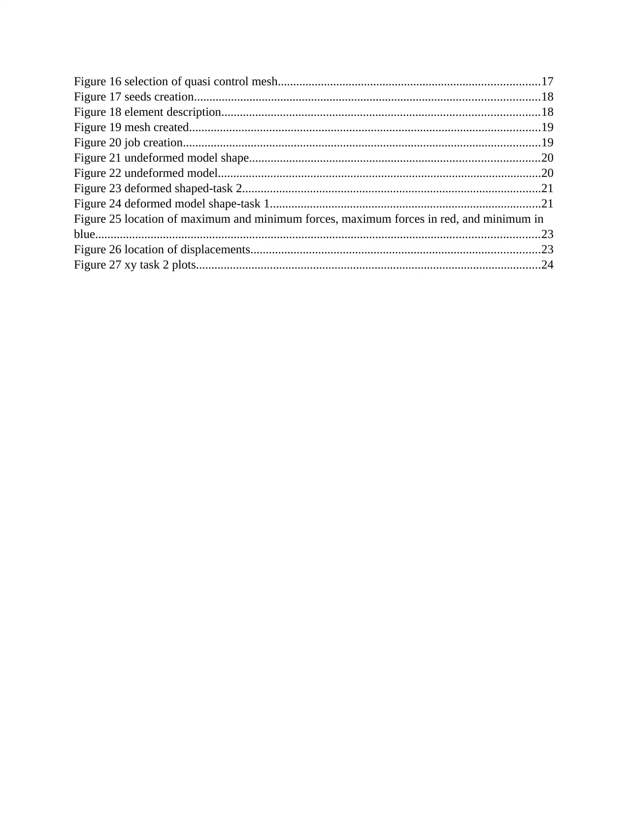
Figure 16 selection of quasi control mesh.....................................................................................17
Figure 17 seeds creation................................................................................................................18
Figure 18 element description.......................................................................................................18
Figure 19 mesh created..................................................................................................................19
Figure 20 job creation....................................................................................................................19
Figure 21 undeformed model shape..............................................................................................20
Figure 22 undeformed model.........................................................................................................20
Figure 23 deformed shaped-task 2.................................................................................................21
Figure 24 deformed model shape-task 1........................................................................................21
Figure 25 location of maximum and minimum forces, maximum forces in red, and minimum in
blue................................................................................................................................................23
Figure 26 location of displacements..............................................................................................23
Figure 27 xy task 2 plots................................................................................................................24

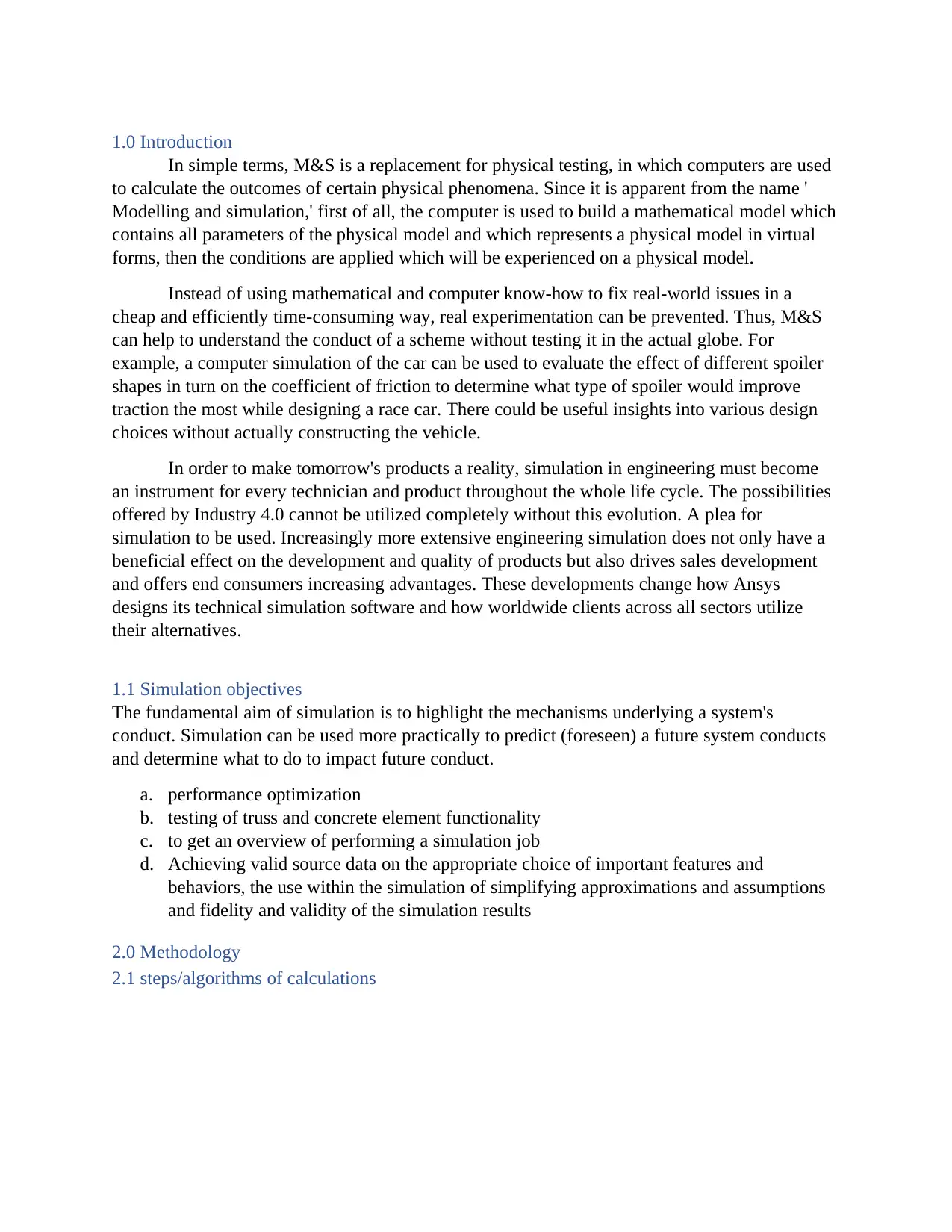
1.0 Introduction
In simple terms, M&S is a replacement for physical testing, in which computers are used
to calculate the outcomes of certain physical phenomena. Since it is apparent from the name '
Modelling and simulation,' first of all, the computer is used to build a mathematical model which
contains all parameters of the physical model and which represents a physical model in virtual
forms, then the conditions are applied which will be experienced on a physical model.
Instead of using mathematical and computer know-how to fix real-world issues in a
cheap and efficiently time-consuming way, real experimentation can be prevented. Thus, M&S
can help to understand the conduct of a scheme without testing it in the actual globe. For
example, a computer simulation of the car can be used to evaluate the effect of different spoiler
shapes in turn on the coefficient of friction to determine what type of spoiler would improve
traction the most while designing a race car. There could be useful insights into various design
choices without actually constructing the vehicle.
In order to make tomorrow's products a reality, simulation in engineering must become
an instrument for every technician and product throughout the whole life cycle. The possibilities
offered by Industry 4.0 cannot be utilized completely without this evolution. A plea for
simulation to be used. Increasingly more extensive engineering simulation does not only have a
beneficial effect on the development and quality of products but also drives sales development
and offers end consumers increasing advantages. These developments change how Ansys
designs its technical simulation software and how worldwide clients across all sectors utilize
their alternatives.
1.1 Simulation objectives
The fundamental aim of simulation is to highlight the mechanisms underlying a system's
conduct. Simulation can be used more practically to predict (foreseen) a future system conducts
and determine what to do to impact future conduct.
a. performance optimization
b. testing of truss and concrete element functionality
c. to get an overview of performing a simulation job
d. Achieving valid source data on the appropriate choice of important features and
behaviors, the use within the simulation of simplifying approximations and assumptions
and fidelity and validity of the simulation results
2.0 Methodology
2.1 steps/algorithms of calculations

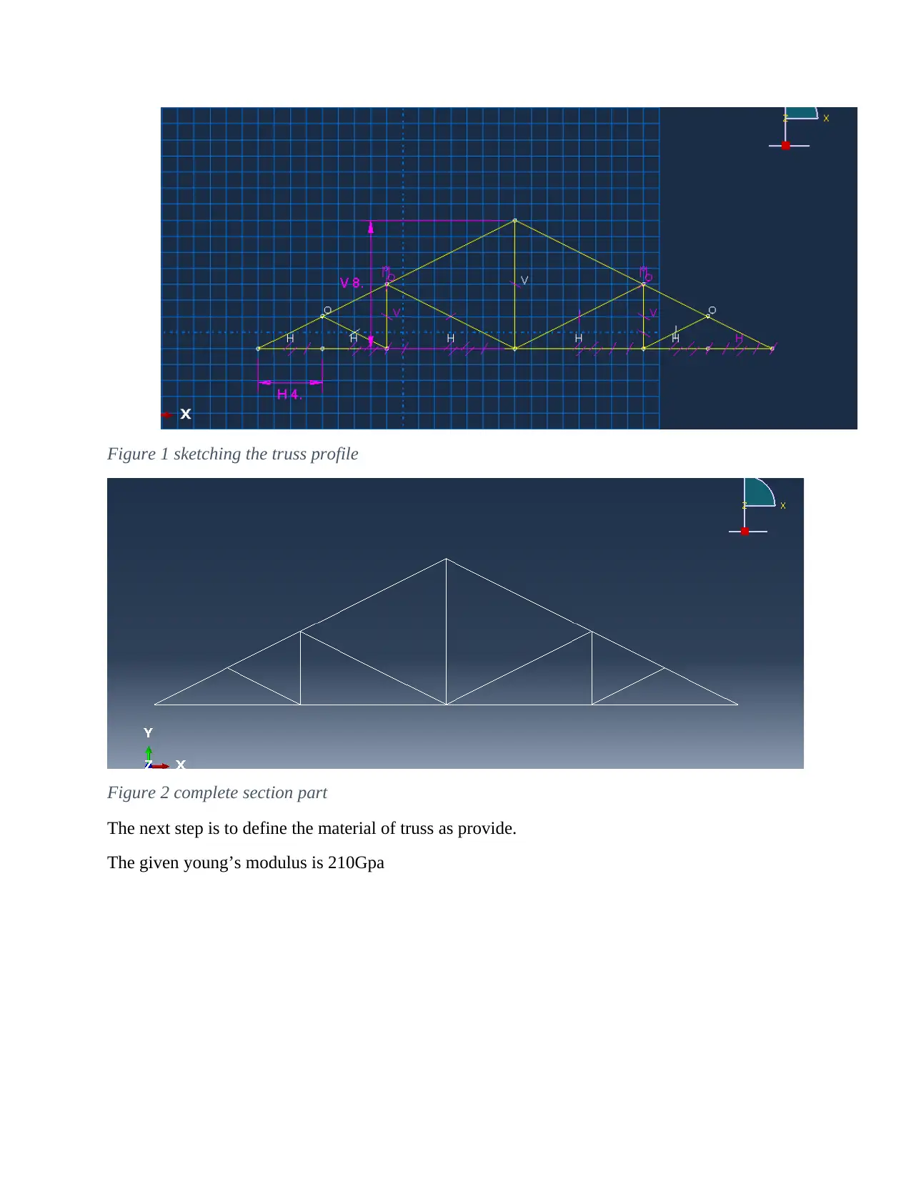
Figure 1 sketching the truss profile
Figure 2 complete section part
The next step is to define the material of truss as provide.
The given young’s modulus is 210Gpa

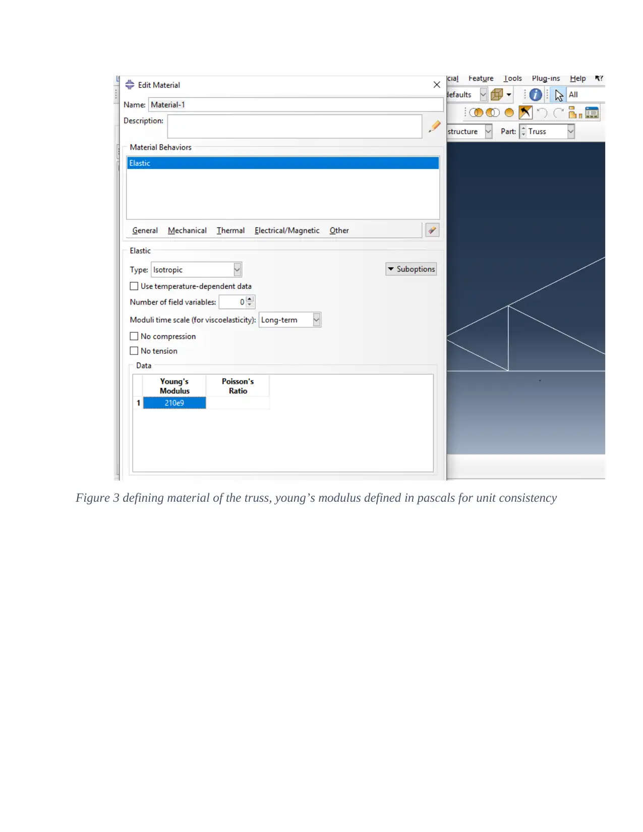
Figure 3 defining material of the truss, young’s modulus defined in pascals for unit consistency

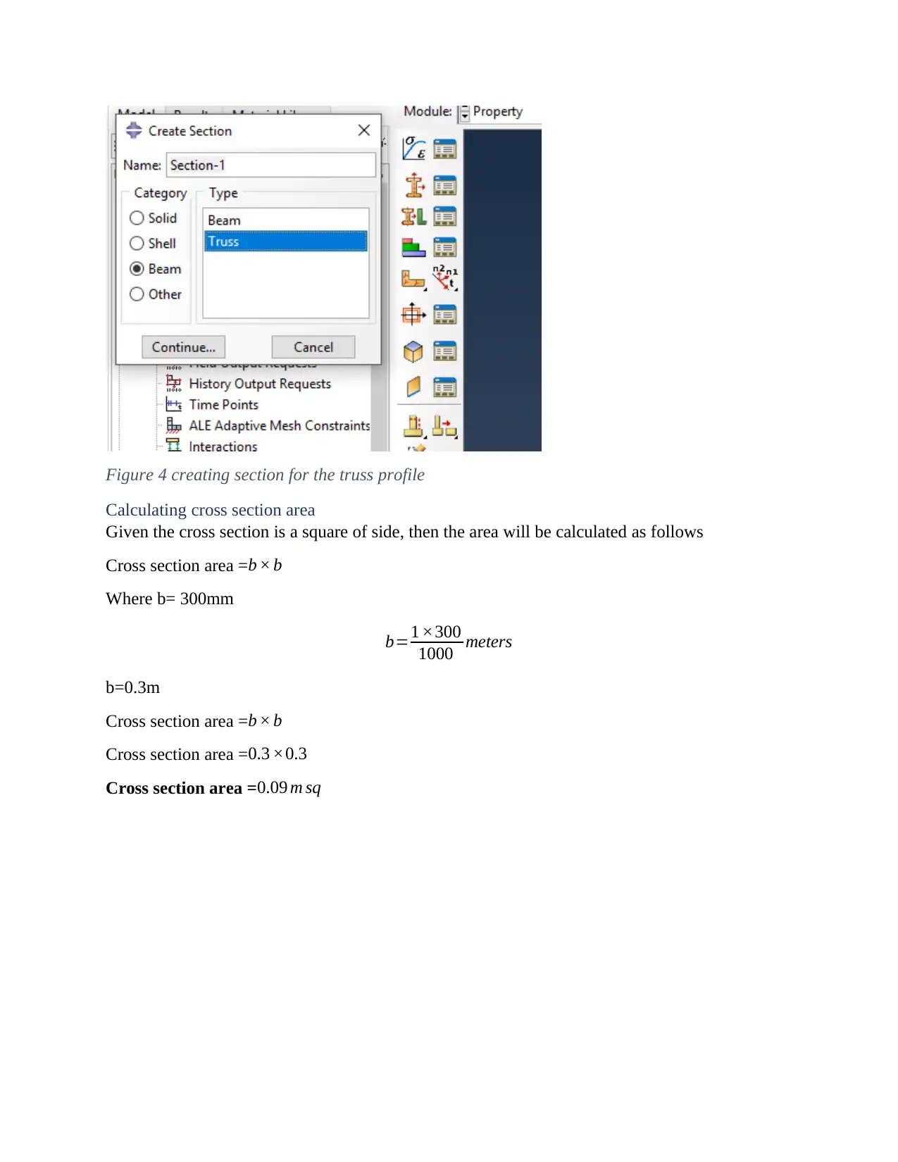
Figure 4 creating section for the truss profile
Calculating cross section area
Given the cross section is a square of side, then the area will be calculated as follows
Cross section area =b × b
Where b= 300mm
b=1 ×300
1000 meters
b=0.3m
Cross section area =b × b
Cross section area =0.3 ×0.3
Cross section area =0.09 m sq

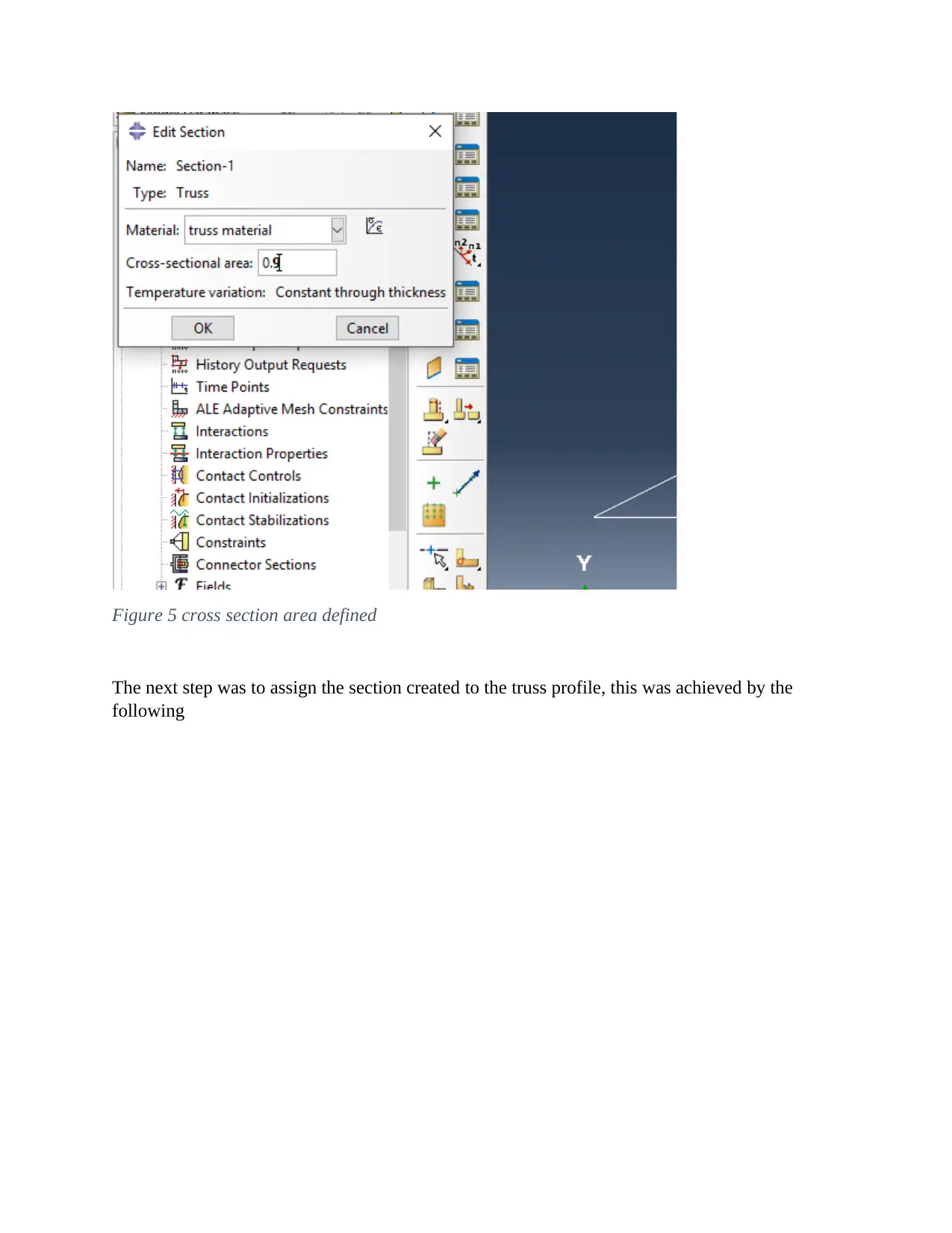
Figure 5 cross section area defined
The next step was to assign the section created to the truss profile, this was achieved by the
following

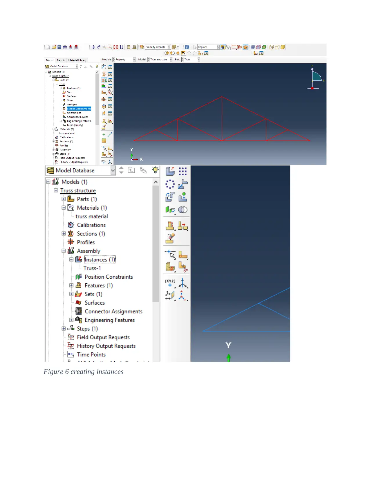
Figure 6 creating instances

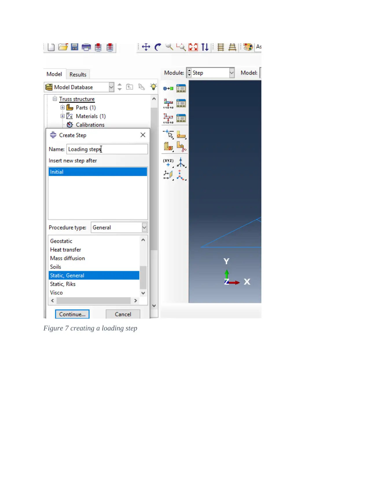
Figure 7 creating a loading step

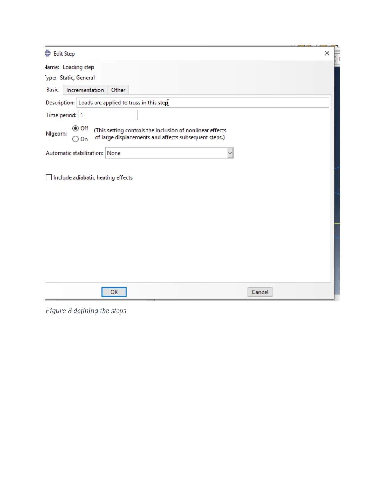
Figure 8 defining the steps

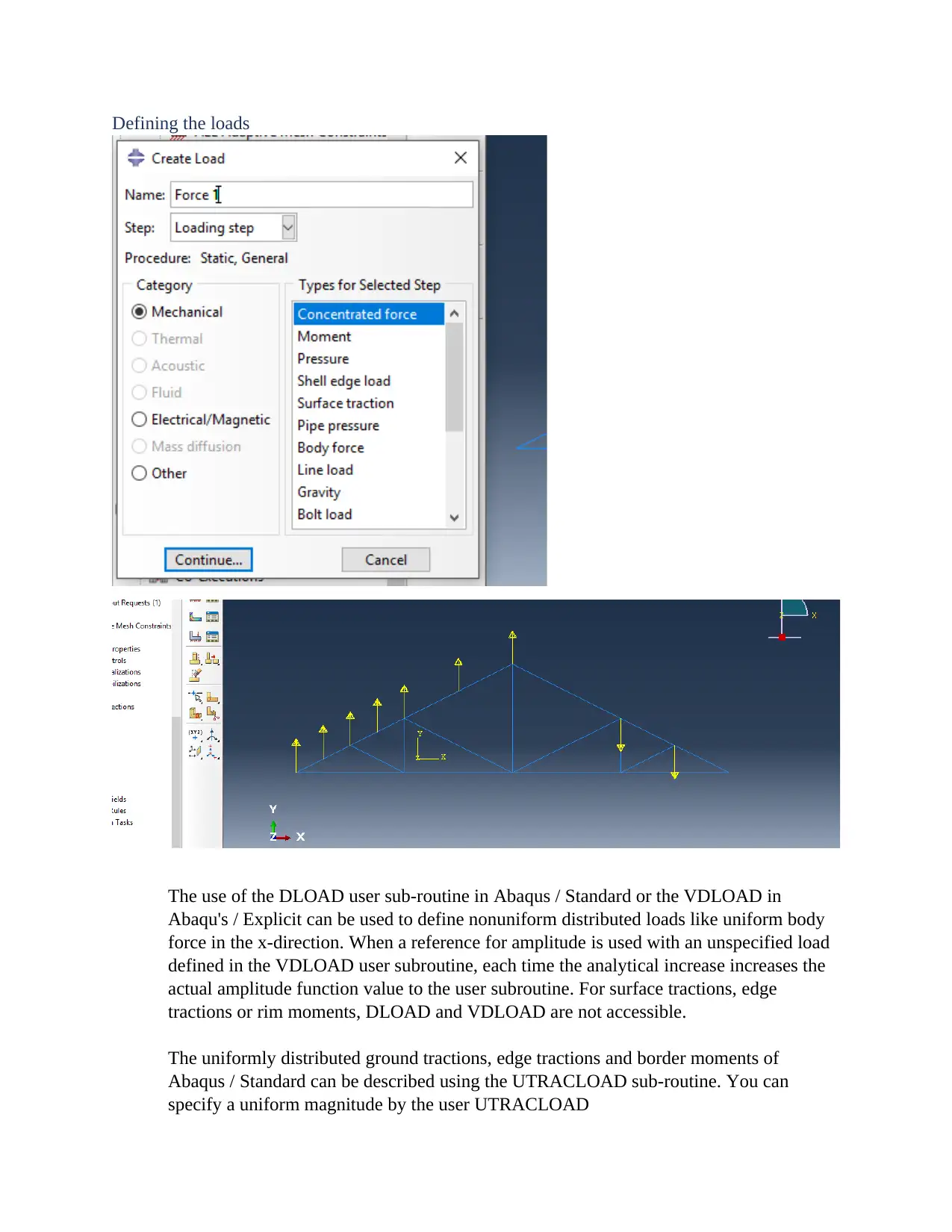
Defining the loads
The use of the DLOAD user sub-routine in Abaqus / Standard or the VDLOAD in
Abaqu's / Explicit can be used to define nonuniform distributed loads like uniform body
force in the x-direction. When a reference for amplitude is used with an unspecified load
defined in the VDLOAD user subroutine, each time the analytical increase increases the
actual amplitude function value to the user subroutine. For surface tractions, edge
tractions or rim moments, DLOAD and VDLOAD are not accessible.
The uniformly distributed ground tractions, edge tractions and border moments of
Abaqus / Standard can be described using the UTRACLOAD sub-routine. You can
specify a uniform magnitude by the user UTRACLOAD