Biomechanics of Sport and Exercise
VerifiedAdded on 2023/03/23
|39
|4615
|27
AI Summary
This document is a case study on the relationship between the technical application of force and sprint start performance measures in the field of sport and exercise science. It includes calculations, explanations, and discussions on various biomechanical variables and their implications in sprinting. The study also investigates the differences in running techniques with induced leg length discrepancy.
Contribute Materials
Your contribution can guide someone’s learning journey. Share your
documents today.

MODULE CODE: 66-500415
SEMESTER TWO EXAMINATION-MAY 2019
MAIN
FACULTY: Health and Wellbeing
DEPARTMENT: Academy of Sport and Physical Activity
MODULE TITLE: Biomechanics of Sport and Exercise
MODULE LEADER: Dr Andrew Barnes
TIME ALLOWED: 2 hours (plus 10 minutes reading time)
___________________________________________________________________
EXAMINATIONCONDUCT:
1. The Examination Conduct Policy outlines the behavioural expectations of
candidates attending any examination.
2. It is a fundamental principle that students are assessed fairly and equitably. The
University Academic Conduct Regulation defines unfair behaviour relating to an
examination to be 'cheating'. The University will investigate and may sanction any
acts or behaviours which breach the Code of Academic Conduct.
INSTRUCTIONS TO CANDIDATES:
1. Please do NOT start writing until told to do so by the invigilator.
2. Candidates must NOT use red ink on the script answer book.
3. Candidates will bring their own calculator. Calculators must display a SHU approved
sticker (red).
4. Candidates SHOULD answer ALL questions on the paper. ALL answers
SHOULD be written within this question paper.
5. This is a CLOSED BOOK examination. NO material may be taken into the
examination.
6. This examination paper MAY NOTbe taken from the venue by the candidates.
7. Please write yourSTUDENT ID/DESK NOhere:__________________/_______
_____________________________________________________________________
STATIONERY REQUIREMENTS PER CANDIDATE:
1 x Anonymous Front Cover Sheet
_____________________________________________________________________
THIS PAPER CONTAINS 39 PAGES INCLUDING THIS SHEET Page 1 of 39
Secure Best Marks with AI Grader
Need help grading? Try our AI Grader for instant feedback on your assignments.

MODULE CODE: 66-500415
This is a blank page
Page 2 of 39
This is a blank page
Page 2 of 39
MODULE CODE: 66-500415
CASE STUDY ONE - (31marks)
Case-study one investigated the relationship between the technical application of force
and commonly used sprint start performance measures in a group of sport and exercise
science students. Thirty nine students performed a 30m sprint from a crouched start, off
a force platform with split times measured at 10, 20 and 30m.
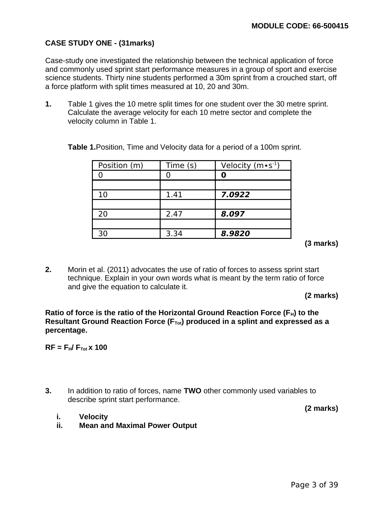
1. Table 1 gives the 10 metre split times for one student over the 30 metre sprint.
Calculate the average velocity for each 10 metre sector and complete the
velocity column in Table 1.
Table 1.Position, Time and Velocity data for a period of a 100m sprint.
Position (m) Time (s) Velocity (m∙s-1)
0 0 0
10 1.41 7.0922
20 2.47 8.097
30 3.34 8.9820
(3 marks)
2. Morin et al. (2011) advocates the use of ratio of forces to assess sprint start
technique. Explain in your own words what is meant by the term ratio of force
and give the equation to calculate it.
(2 marks)
Ratio of force is the ratio of the Horizontal Ground Reaction Force (FH) to the
Resultant Ground Reaction Force (FTot) produced in a splint and expressed as a
percentage.
RF = FH/ FTot x 100
3. In addition to ratio of forces, name TWO other commonly used variables to
describe sprint start performance.
(2 marks)
i. Velocity
ii. Mean and Maximal Power Output
Page 3 of 39
CASE STUDY ONE - (31marks)
Case-study one investigated the relationship between the technical application of force
and commonly used sprint start performance measures in a group of sport and exercise
science students. Thirty nine students performed a 30m sprint from a crouched start, off
a force platform with split times measured at 10, 20 and 30m.
1. Table 1 gives the 10 metre split times for one student over the 30 metre sprint.
Calculate the average velocity for each 10 metre sector and complete the
velocity column in Table 1.
Table 1.Position, Time and Velocity data for a period of a 100m sprint.
Position (m) Time (s) Velocity (m∙s-1)
0 0 0
10 1.41 7.0922
20 2.47 8.097
30 3.34 8.9820
(3 marks)
2. Morin et al. (2011) advocates the use of ratio of forces to assess sprint start
technique. Explain in your own words what is meant by the term ratio of force
and give the equation to calculate it.
(2 marks)
Ratio of force is the ratio of the Horizontal Ground Reaction Force (FH) to the
Resultant Ground Reaction Force (FTot) produced in a splint and expressed as a
percentage.
RF = FH/ FTot x 100
3. In addition to ratio of forces, name TWO other commonly used variables to
describe sprint start performance.
(2 marks)
i. Velocity
ii. Mean and Maximal Power Output
Page 3 of 39

MODULE CODE: 66-500415
Page 4 of 39
Page 4 of 39
Secure Best Marks with AI Grader
Need help grading? Try our AI Grader for instant feedback on your assignments.
MODULE CODE: 66-500415
4. This data collection used a force platform to capture ground reaction forces
during the push off phase of the sprint start. Give three limitations of using a
force platform to capture ground reaction force data.
(3 marks)
i. They are not very accurate
ii. They are expensive
iii. The subjects have to step on the plates with force.
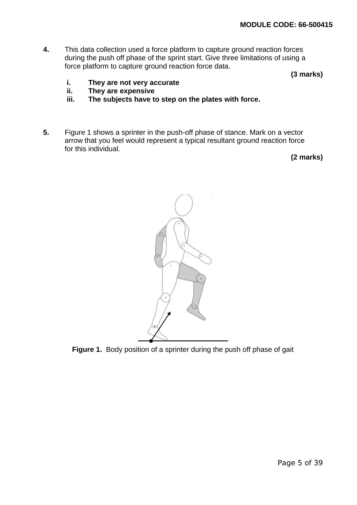
5. Figure 1 shows a sprinter in the push-off phase of stance. Mark on a vector
arrow that you feel would represent a typical resultant ground reaction force
for this individual.
(2 marks)
Figure 1. Body position of a sprinter during the push off phase of gait
Page 5 of 39
4. This data collection used a force platform to capture ground reaction forces
during the push off phase of the sprint start. Give three limitations of using a
force platform to capture ground reaction force data.
(3 marks)
i. They are not very accurate
ii. They are expensive
iii. The subjects have to step on the plates with force.
5. Figure 1 shows a sprinter in the push-off phase of stance. Mark on a vector
arrow that you feel would represent a typical resultant ground reaction force
for this individual.
(2 marks)
Figure 1. Body position of a sprinter during the push off phase of gait
Page 5 of 39

MODULE CODE: 66-500415
6. Table 2 contains horizontal force data for a 68 kg student during the push off
phase of a sprint start, captured using a force plate. Using the equations
provided, calculate the impulse and the associated change in velocity over
this period.
Table 2.Horizontal Forces generated during the push off phase of a sprint start
Time (s) Horizontal Force (N)
0.001 22.82
0.002 23.43
0.003 25.26
0.004 26.72
0.005 29.23
0.006 31.60
0.007 33.96
0.008 35.34
(6 marks)
Impulse = Force (N) x Time (s)
Time (s) Horizontal Force (N) Impulse (Ns)
0.001 22.82 0.02282
0.002 23.43 0.04686
0.003 25.26 0.07578
0.004 26.72 0.10688
0.005 29.23 0.14615
0.006 31.6 0.1896
0.007 33.96 0.23772
0.008 35.34 0.28272
Page 6 of 39
MODULE CODE: 66-500415
Associated Change in Velocity = Final Velocity (Vf) – Initial Velocity (Vi)
= 0.28272/68000 - 0.02282/68000
= 8.0176 x 10-07m/s
Page 7 of 39
Associated Change in Velocity = Final Velocity (Vf) – Initial Velocity (Vi)
= 0.28272/68000 - 0.02282/68000
= 8.0176 x 10-07m/s
Page 7 of 39
Paraphrase This Document
Need a fresh take? Get an instant paraphrase of this document with our AI Paraphraser
MODULE CODE: 66-500415
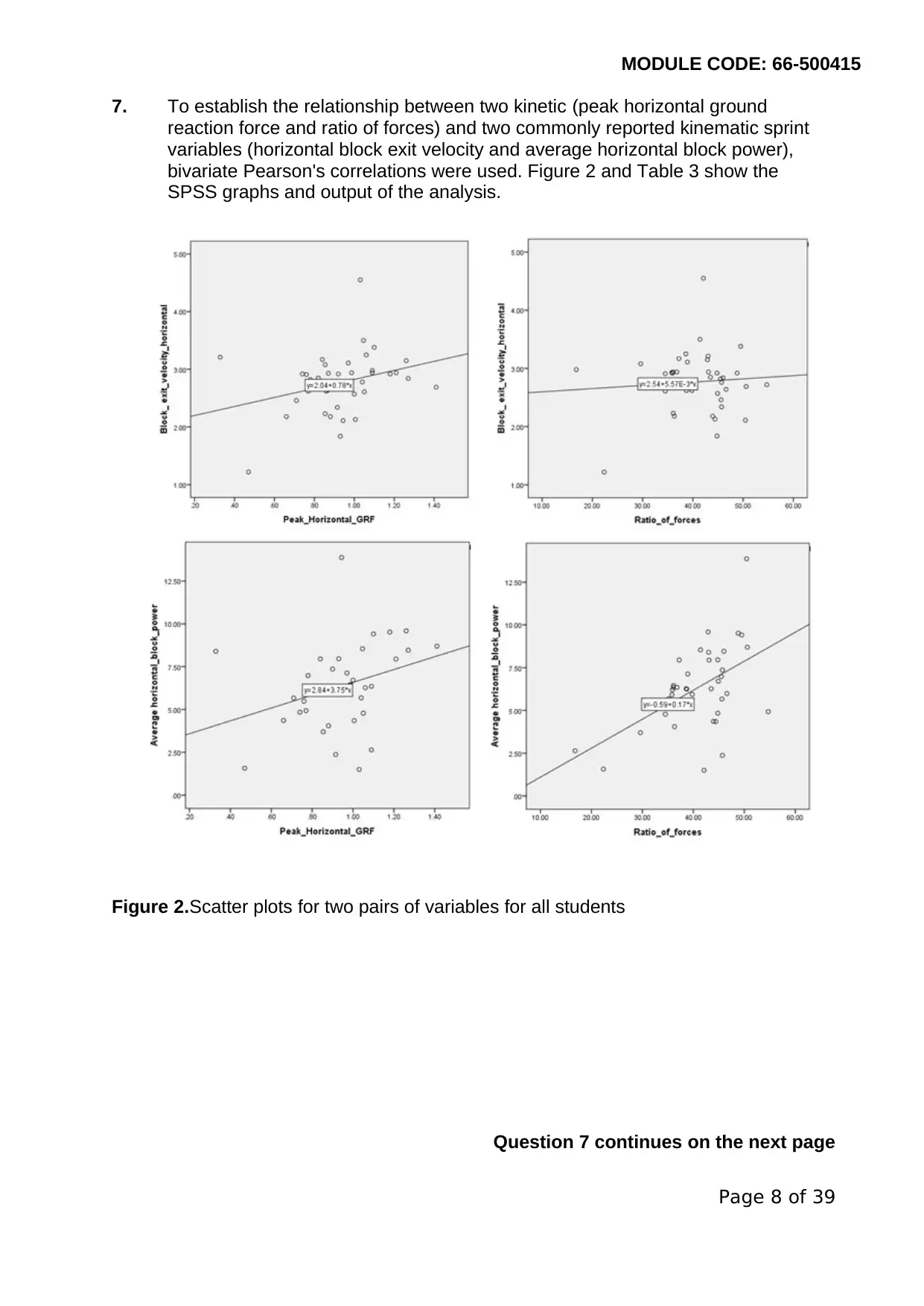
7. To establish the relationship between two kinetic (peak horizontal ground
reaction force and ratio of forces) and two commonly reported kinematic sprint
variables (horizontal block exit velocity and average horizontal block power),
bivariate Pearson's correlations were used. Figure 2 and Table 3 show the
SPSS graphs and output of the analysis.
Figure 2.Scatter plots for two pairs of variables for all students
Question 7 continues on the next page
Page 8 of 39
MODULE CODE: 66-500415
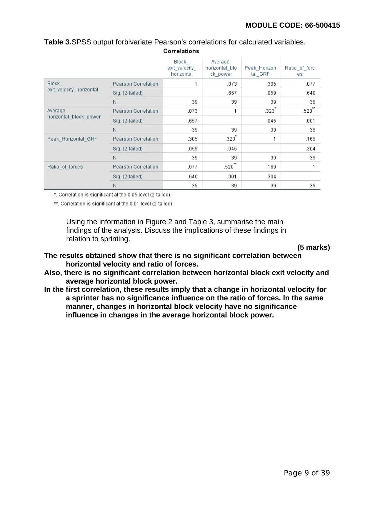
Table 3.SPSS output forbivariate Pearson's correlations for calculated variables.
Using the information in Figure 2 and Table 3, summarise the main
findings of the analysis. Discuss the implications of these findings in
relation to sprinting.
(5 marks)
The results obtained show that there is no significant correlation between
horizontal velocity and ratio of forces.
Also, there is no significant correlation between horizontal block exit velocity and
average horizontal block power.
In the first correlation, these results imply that a change in horizontal velocity for
a sprinter has no significance influence on the ratio of forces. In the same
manner, changes in horizontal block velocity have no significance
influence in changes in the average horizontal block power.
Page 9 of 39

MODULE CODE: 66-500415
Page 10 of 39
Page 10 of 39
Secure Best Marks with AI Grader
Need help grading? Try our AI Grader for instant feedback on your assignments.
MODULE CODE: 66-500415
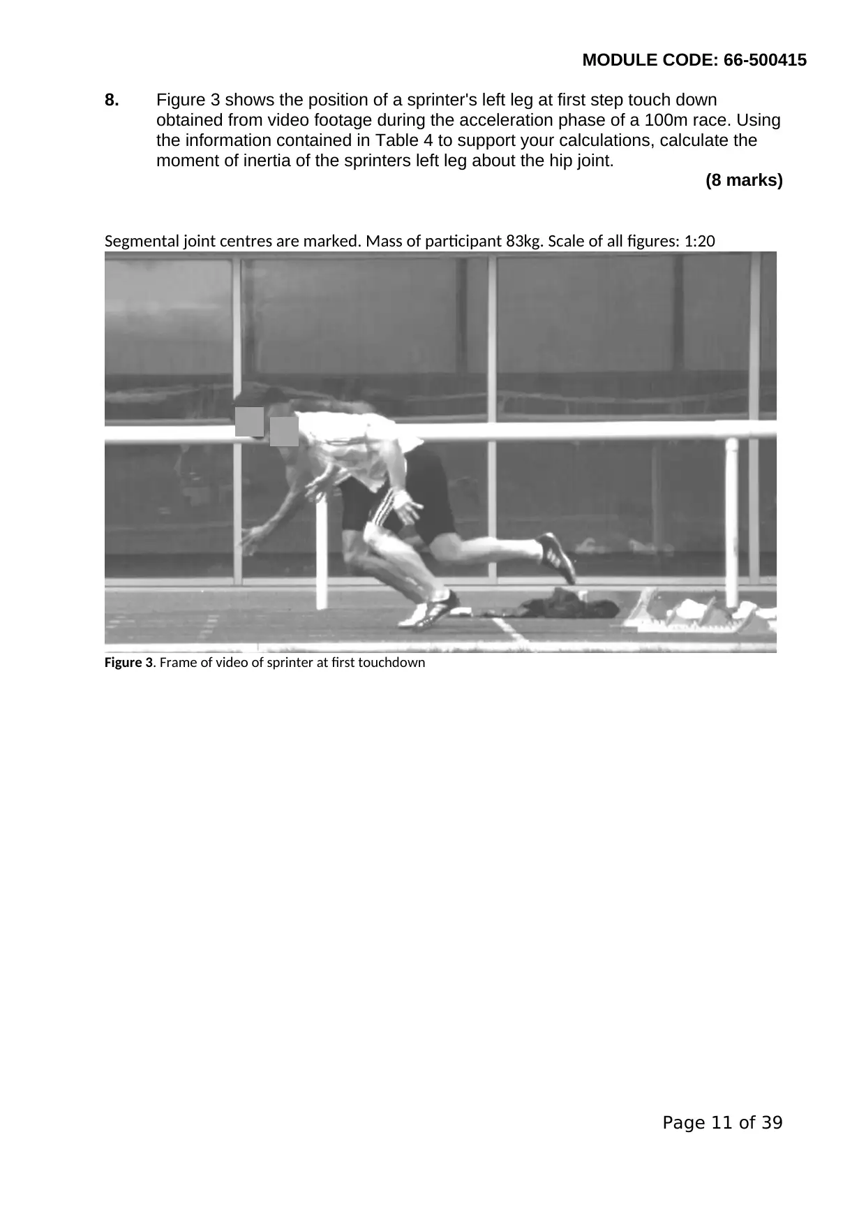
8. Figure 3 shows the position of a sprinter's left leg at first step touch down
obtained from video footage during the acceleration phase of a 100m race. Using
the information contained in Table 4 to support your calculations, calculate the
moment of inertia of the sprinters left leg about the hip joint.
(8 marks)
Segmental joint centres are marked. Mass of participant 83kg. Scale of all figures: 1:20
Figure 3. Frame of video of sprinter at first touchdown
Page 11 of 39
MODULE CODE: 66-500415
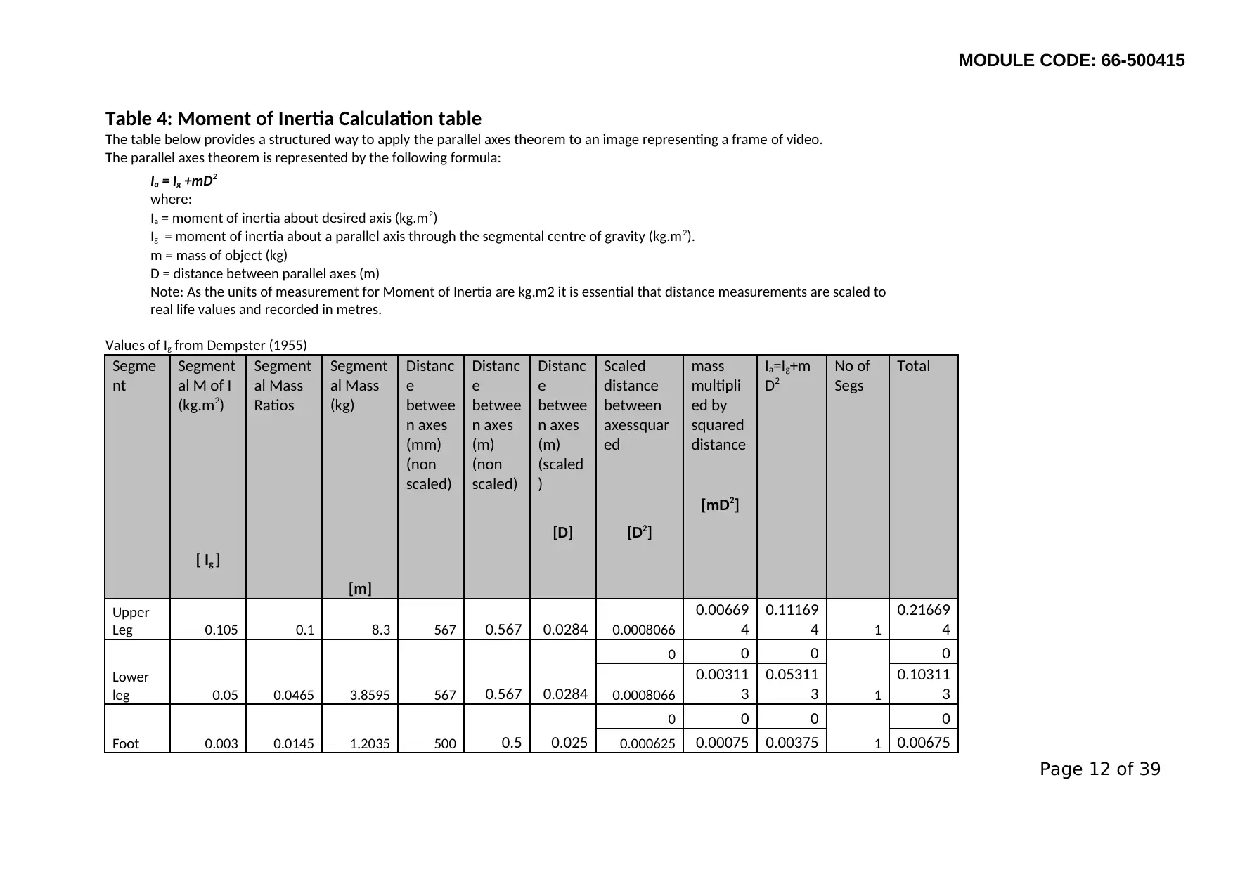
Table 4: Moment of Inertia Calculation table
The table below provides a structured way to apply the parallel axes theorem to an image representing a frame of video.
The parallel axes theorem is represented by the following formula:
Ia = Ig +mD2
where:
Ia = moment of inertia about desired axis (kg.m2)
Ig = moment of inertia about a parallel axis through the segmental centre of gravity (kg.m2).
m = mass of object (kg)
D = distance between parallel axes (m)
Note: As the units of measurement for Moment of Inertia are kg.m2 it is essential that distance measurements are scaled to
real life values and recorded in metres.
Values of Ig from Dempster (1955)
Segme
nt
Segment
al M of I
(kg.m2)
Segment
al Mass
Ratios
Segment
al Mass
(kg)
Distanc
e
betwee
n axes
(mm)
(non
scaled)
Distanc
e
betwee
n axes
(m)
(non
scaled)
Distanc
e
betwee
n axes
(m)
(scaled
)
Scaled
distance
between
axessquar
ed
mass
multipli
ed by
squared
distance
Ia=Ig+m
D2
No of
Segs
Total
[mD2]
[D] [D2]
[ Ig ]
[m]
Upper
Leg 0.105 0.1 8.3 567 0.567 0.0284 0.0008066
0.00669
4
0.11169
4 1
0.21669
4
Lower
leg 0.0465
0 0 0
1
0
0.05 3.8595 567 0.567 0.0284 0.0008066
0.00311
3
0.05311
3
0.10311
3
Foot 0.0145
0 0 0
1
0
0.003 1.2035 500 0.5 0.025 0.000625 0.00075 0.00375 0.00675
Page 12 of 39
MODULE CODE: 66-500415
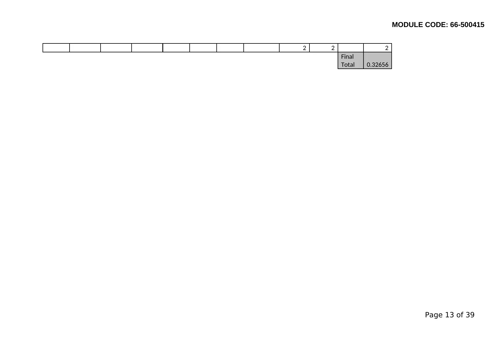
2 2 2
Final
Total 0.32656
Page 13 of 39
2 2 2
Final
Total 0.32656
Page 13 of 39
Paraphrase This Document
Need a fresh take? Get an instant paraphrase of this document with our AI Paraphraser
MODULE CODE: 66-500415
CASE STUDY TWO - (38 marks)
Casestudy two investigated differences in temporal and kinematic variables when
running with and without induced leg length discrepancy. Participants were asked to run
on a treadmill at a self-selected speed wearing specially adapted footwear to induce a
leg length discrepancy.This was then repeated while wearing their normal footwear. 2D
video was captured in the sagittal plane for both conditionsto allow a comparison of the
associated running techniques.
9. During this data collection, the camera used a frame rate of 50Hz and a shutter
speed of 1/500. Explain difference between the frame rate and the shutter speed
on a camera what the shutter speed on the camera controls?
(2 marks)
Frame rate is the camera’s speed in capturing photos while shutter speed is the
speed is the length for which the shutter remains open after a photo has been
captured.
Shutter speed controls the amount of light going to the sensor.
10. There are numerous potential sources of error in the capture and processing
of 2D video. List two possible sources of random error in this process?
(2 marks)
i. Placement of markers
ii. Digitization of markers
11. The stance time for a given running cycle was recorded as 0.31 seconds and
the total cycle time as 0.82 seconds. Calculate the contact and non-contact
time expressed as a percentage of the total running cycle.
(3 marks)
Total Running Cycle = Stance Time + Total cycle Time
= 0.31 + 0.82
= 1.13 seconds
Contact time = 0.31/1.13 x 100 = 27.43%
Page 14 of 39

MODULE CODE: 66-500415
Non-contact time = 0.82/1.13 x 100%
= 72.57%
Page 15 of 39
Non-contact time = 0.82/1.13 x 100%
= 72.57%
Page 15 of 39
MODULE CODE: 66-500415
12. (a) What equation relates running speed, stride length and stride
frequency.
(2 marks)
Running Speed = Stride Length x Stride Frequency
V = SL x SF
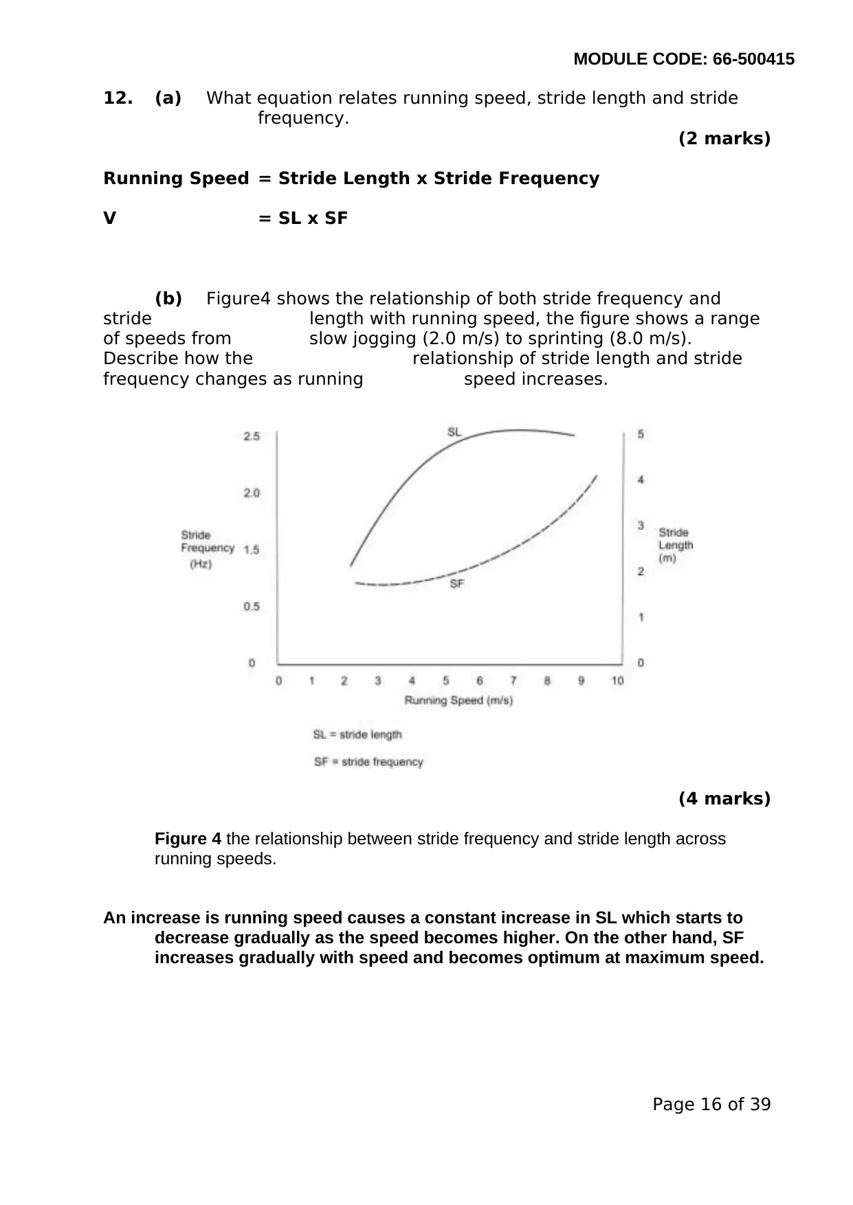
(b) Figure4 shows the relationship of both stride frequency and
stride length with running speed, the figure shows a range
of speeds from slow jogging (2.0 m/s) to sprinting (8.0 m/s).
Describe how the relationship of stride length and stride
frequency changes as running speed increases.
(4 marks)
Figure 4 the relationship between stride frequency and stride length across
running speeds.
An increase is running speed causes a constant increase in SL which starts to
decrease gradually as the speed becomes higher. On the other hand, SF
increases gradually with speed and becomes optimum at maximum speed.
Page 16 of 39
12. (a) What equation relates running speed, stride length and stride
frequency.
(2 marks)
Running Speed = Stride Length x Stride Frequency
V = SL x SF
(b) Figure4 shows the relationship of both stride frequency and
stride length with running speed, the figure shows a range
of speeds from slow jogging (2.0 m/s) to sprinting (8.0 m/s).
Describe how the relationship of stride length and stride
frequency changes as running speed increases.
(4 marks)
Figure 4 the relationship between stride frequency and stride length across
running speeds.
An increase is running speed causes a constant increase in SL which starts to
decrease gradually as the speed becomes higher. On the other hand, SF
increases gradually with speed and becomes optimum at maximum speed.
Page 16 of 39
Secure Best Marks with AI Grader
Need help grading? Try our AI Grader for instant feedback on your assignments.
MODULE CODE: 66-500415
13. To investigate kinematic differences associated with induced leg length
discrepancy, key angles of the lower extremity may be calculated. The data in
Table 5 shows joint positions from a participant's left leg for a single frame of
video.
Table 5. The data is for the left leg for a single video frame with the runner
travelling from right to left. (Note: that the x coordinate refers to the horizontal
measurement and the y coordinate refers to the vertical measurement in the
2D plane).
Hip
x coordinate
(mm)
Hip
y coordinate
(mm)
Knee
x coordinate
(mm)
Knee
y coordinate
(mm)
Ankle
x coordinate
(mm)
Ankle
y coordinate
(mm)
372.00 955.00 205.95 457.05 580.90 355.98
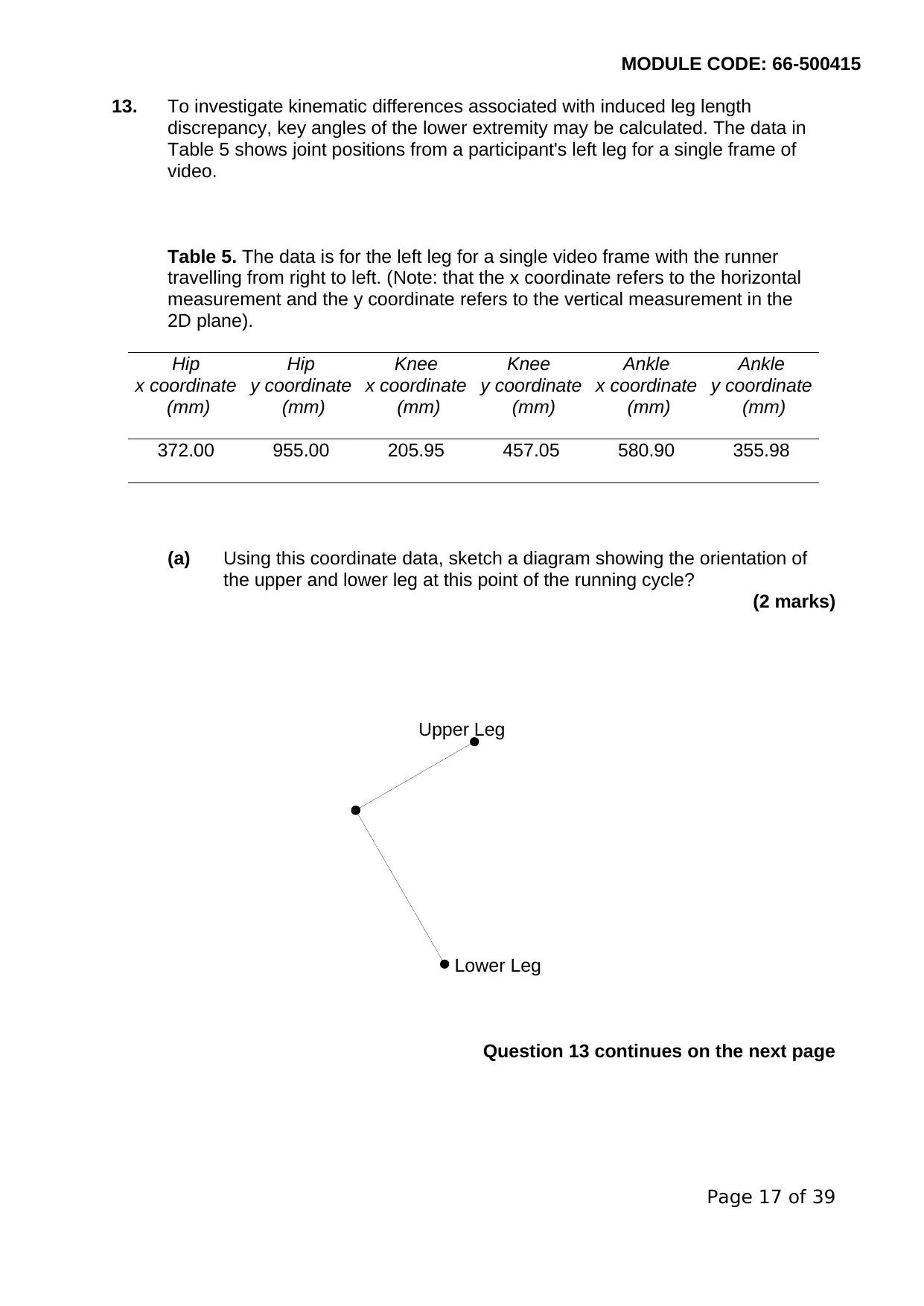
(a) Using this coordinate data, sketch a diagram showing the orientation of
the upper and lower leg at this point of the running cycle?
(2 marks)
Upper Leg
Lower Leg
Question 13 continues on the next page
Page 17 of 39
13. To investigate kinematic differences associated with induced leg length
discrepancy, key angles of the lower extremity may be calculated. The data in
Table 5 shows joint positions from a participant's left leg for a single frame of
video.
Table 5. The data is for the left leg for a single video frame with the runner
travelling from right to left. (Note: that the x coordinate refers to the horizontal
measurement and the y coordinate refers to the vertical measurement in the
2D plane).
Hip
x coordinate
(mm)
Hip
y coordinate
(mm)
Knee
x coordinate
(mm)
Knee
y coordinate
(mm)
Ankle
x coordinate
(mm)
Ankle
y coordinate
(mm)
372.00 955.00 205.95 457.05 580.90 355.98
(a) Using this coordinate data, sketch a diagram showing the orientation of
the upper and lower leg at this point of the running cycle?
(2 marks)
Upper Leg
Lower Leg
Question 13 continues on the next page
Page 17 of 39
MODULE CODE: 66-500415
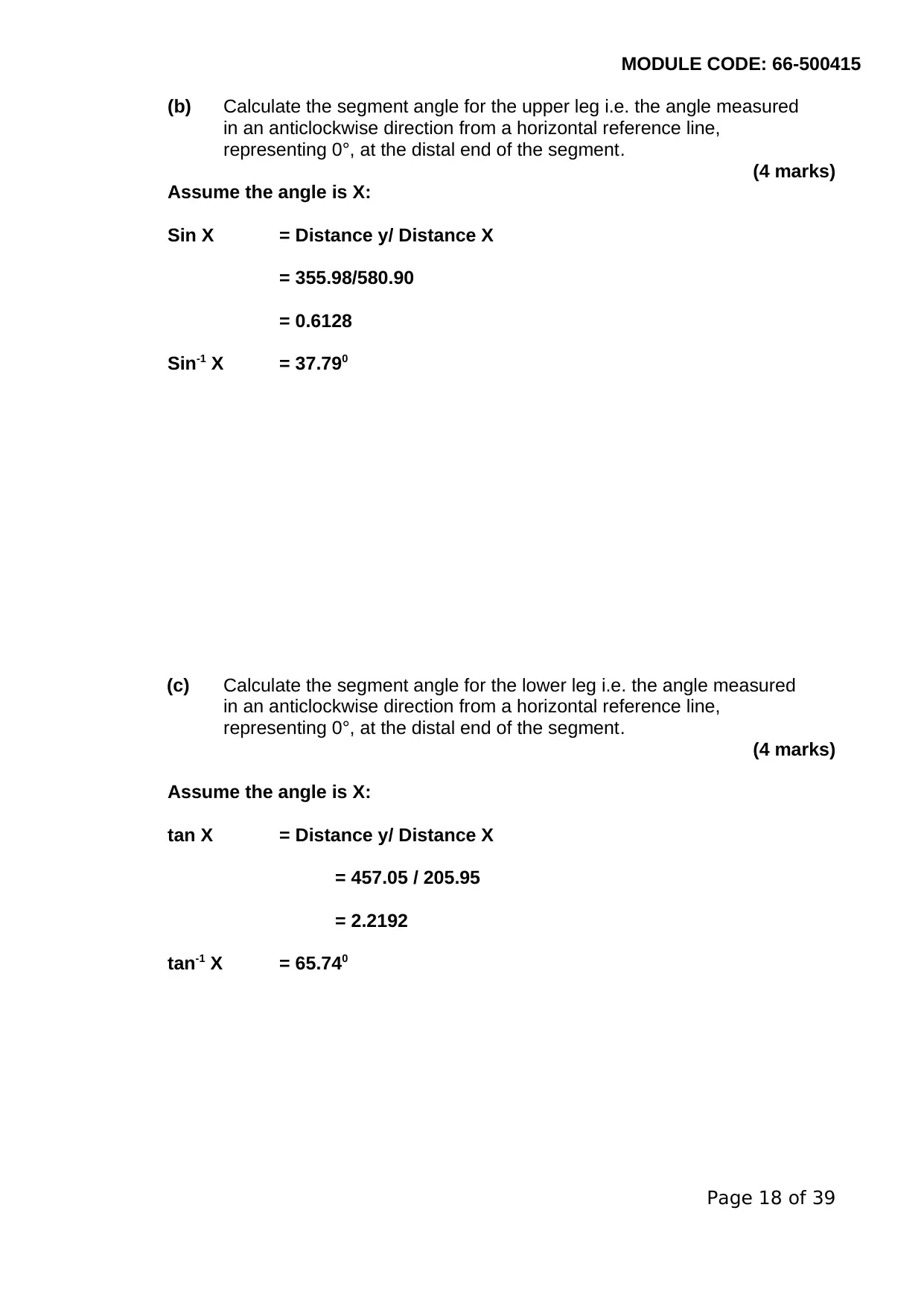
(b) Calculate the segment angle for the upper leg i.e. the angle measured
in an anticlockwise direction from a horizontal reference line,
representing 0°, at the distal end of the segment.
(4 marks)
Assume the angle is X:
Sin X = Distance y/ Distance X
= 355.98/580.90
= 0.6128
Sin-1 X = 37.790
(c) Calculate the segment angle for the lower leg i.e. the angle measured
in an anticlockwise direction from a horizontal reference line,
representing 0°, at the distal end of the segment.
(4 marks)
Assume the angle is X:
tan X = Distance y/ Distance X
= 457.05 / 205.95
= 2.2192
tan-1 X = 65.740
Page 18 of 39

MODULE CODE: 66-500415
Page 19 of 39
Page 19 of 39
Paraphrase This Document
Need a fresh take? Get an instant paraphrase of this document with our AI Paraphraser
MODULE CODE: 66-500415
14.
0 10 20 30 40 50 60 70 80 90 100
0
20
40
60
80
100
120
Knee Angle (°)
Ankle angle (°)
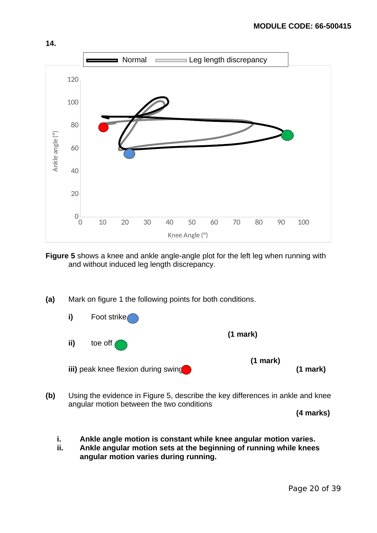
Figure 5 shows a knee and ankle angle-angle plot for the left leg when running with
and without induced leg length discrepancy.
(a) Mark on figure 1 the following points for both conditions.
i) Foot strike
(1 mark)
ii) toe off
(1 mark)
iii) peak knee flexion during swing (1 mark)
(b) Using the evidence in Figure 5, describe the key differences in ankle and knee
angular motion between the two conditions
(4 marks)
i. Ankle angle motion is constant while knee angular motion varies.
ii. Ankle angular motion sets at the beginning of running while knees
angular motion varies during running.
Page 20 of 39
Normal Leg length discrepancy
14.
0 10 20 30 40 50 60 70 80 90 100
0
20
40
60
80
100
120
Knee Angle (°)
Ankle angle (°)
Figure 5 shows a knee and ankle angle-angle plot for the left leg when running with
and without induced leg length discrepancy.
(a) Mark on figure 1 the following points for both conditions.
i) Foot strike
(1 mark)
ii) toe off
(1 mark)
iii) peak knee flexion during swing (1 mark)
(b) Using the evidence in Figure 5, describe the key differences in ankle and knee
angular motion between the two conditions
(4 marks)
i. Ankle angle motion is constant while knee angular motion varies.
ii. Ankle angular motion sets at the beginning of running while knees
angular motion varies during running.
Page 20 of 39
Normal Leg length discrepancy

MODULE CODE: 66-500415
Page 21 of 39
Page 21 of 39

MODULE CODE: 66-500415
15. During running, calculation of a participant's centre of mass is often of interest to
researchers. In order to calculate the centre of mass for the whole body, researchers
often use a process of segmentation which involves calculating the mass and centre of
mass location of individual body segments. The mass and centre of gravity for
individual body segments may be calculated using ratios derived from cadaver data
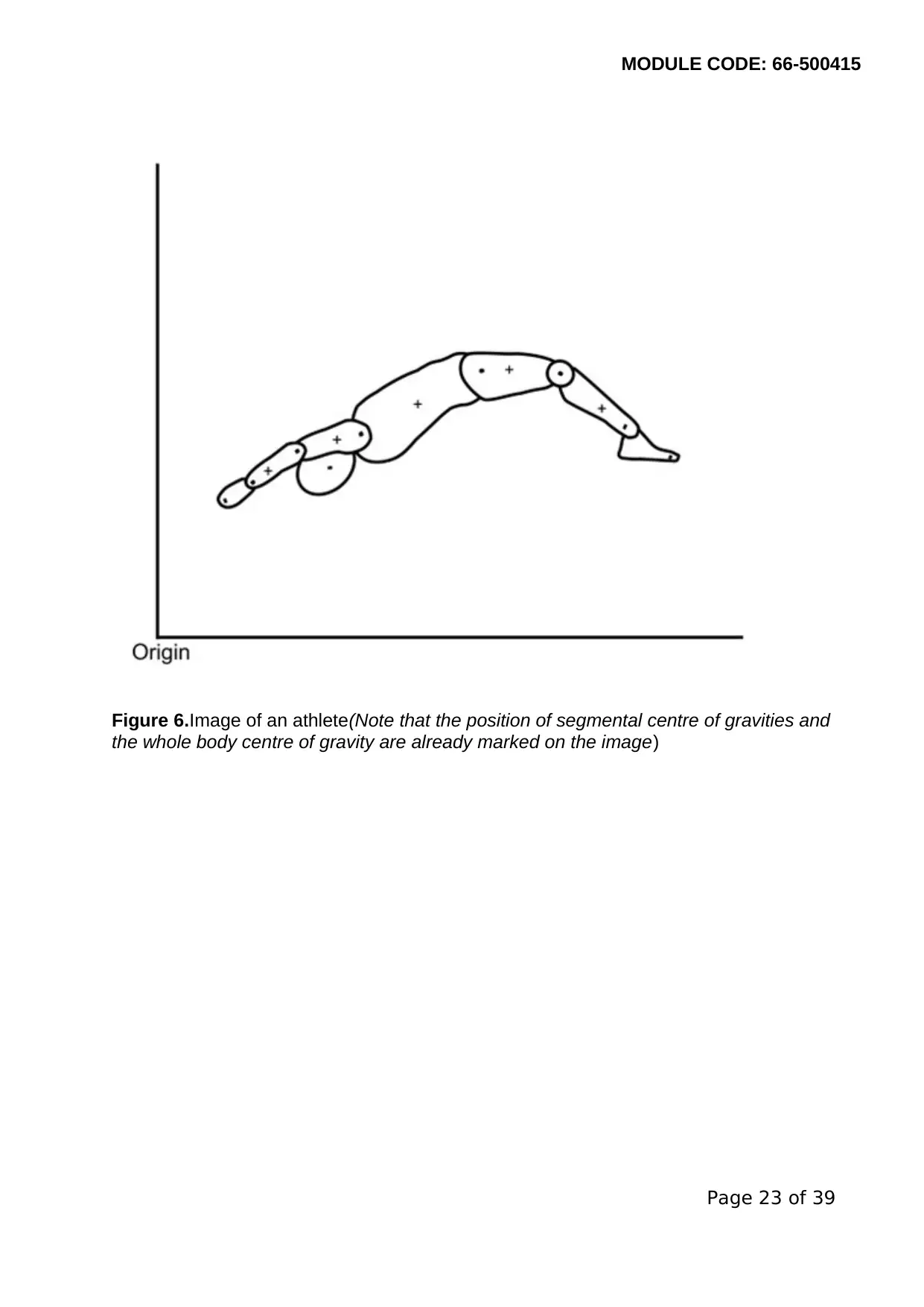
Figure 6 shows the position of an athlete obtained from video footage. You may
assume that the image represents an individual of mass 67 kg in a symmetrical body
position.
The joint centre positions and the segmental centre of gravities have already been
marked on the diagram. Calculate and clearly mark on Figure 6 the position of the
whole body centre of gravity. You must show evidence of your working and complete
Table 6.
(8marks)
Page 22 of 39
15. During running, calculation of a participant's centre of mass is often of interest to
researchers. In order to calculate the centre of mass for the whole body, researchers
often use a process of segmentation which involves calculating the mass and centre of
mass location of individual body segments. The mass and centre of gravity for
individual body segments may be calculated using ratios derived from cadaver data
Figure 6 shows the position of an athlete obtained from video footage. You may
assume that the image represents an individual of mass 67 kg in a symmetrical body
position.
The joint centre positions and the segmental centre of gravities have already been
marked on the diagram. Calculate and clearly mark on Figure 6 the position of the
whole body centre of gravity. You must show evidence of your working and complete
Table 6.
(8marks)
Page 22 of 39
Secure Best Marks with AI Grader
Need help grading? Try our AI Grader for instant feedback on your assignments.
MODULE CODE: 66-500415
Figure 6.Image of an athlete(Note that the position of segmental centre of gravities and
the whole body centre of gravity are already marked on the image)
Page 23 of 39
Figure 6.Image of an athlete(Note that the position of segmental centre of gravities and
the whole body centre of gravity are already marked on the image)
Page 23 of 39
MODULE CODE: 66-500415
Page 24 of 39
A B C D E F G H
SEGMENT Segmenta
l mass
ratio
Product of
Segmental
mass ratio
and total
body
mass (kg)
Segmental
weight
Distance
from
Segmental c
of g to
vertical axis
(mm)
Distance
from
Segmental c
of g to
horizontal
axis (mm)
Product of
D and E
Product
of D and
F
(C* 9.81
N)
Trunk,
head and
neck
0.578 38.726 379.9021 200 250 75980.412 94975.52
Left upper
arm
0.028 1.876 18.40356 150 100 2760.534 1840.356
Right
upper arm
0.028 1.876 18.40356 150 100 2760.534 1840.356
Left lower
arm and
hand
0.022 1.474 14.45994 100 80 1445.994 1156.795
Right
Lower arm
and hand
0.022 1.474 14.45994 100 80 1445.994 1156.795
Left upper
leg
0.1 6.7 65.727 300 350 19718.1 23004.45
Right
upper leg
0.1 6.7 65.727 300 350 19718.1 23004.45
Left lower
leg and
foot
0.061 4.087 40.09347 400 450 16037.388 18042.06
Right
Lower leg
and foot
0.061 4.087 40.09347 400 450 16037.388 18042.06
Sum of Segmental
contributions
155904.4
4
183062.8
Sum of Segmental
Contributions/Weight
237.2 278.52

MODULE CODE: 66-500415
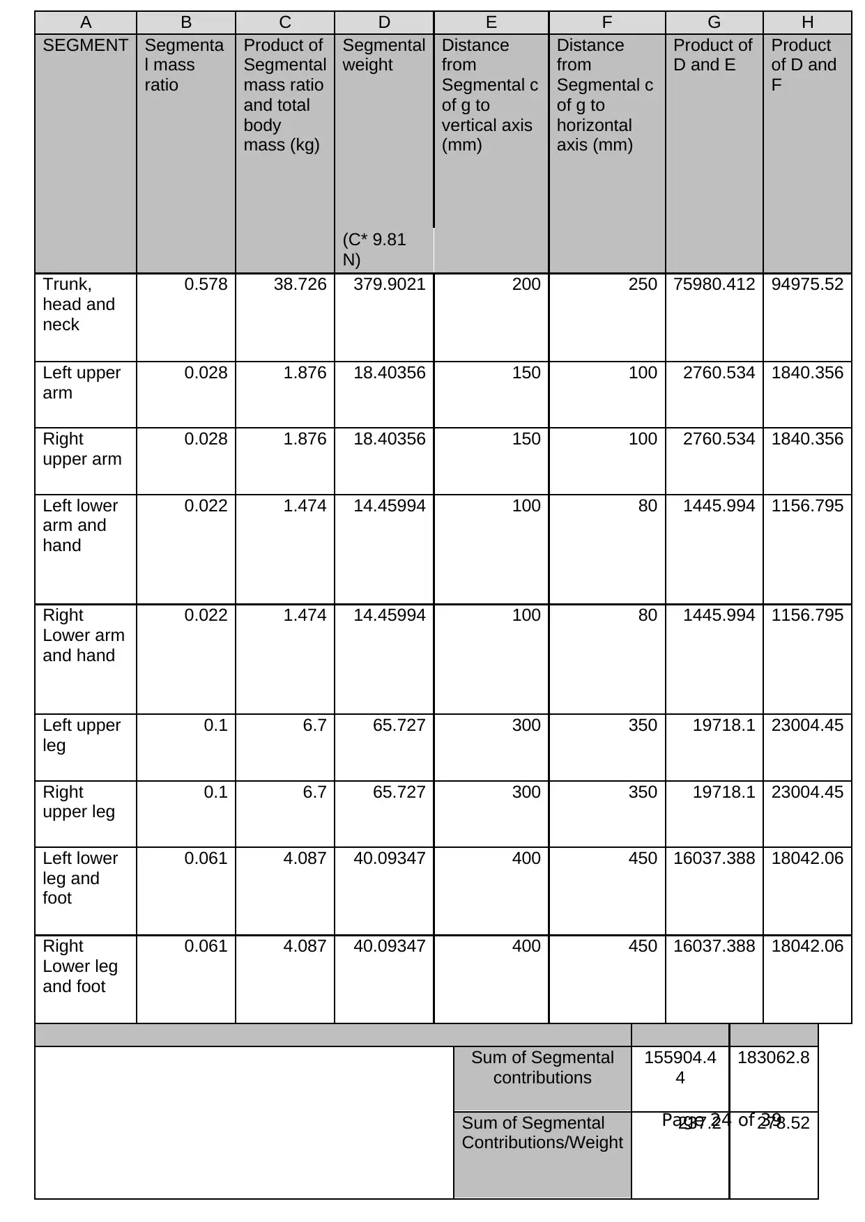
Table 6. Centre of Gravity Table for a 9 segment model
Note: Sum of segmental contributions divided by participant weight gives
two values which equate to the whole body centre of gravity x and y
coordinates measured from the origin.
Page 25 of 39
Table 6. Centre of Gravity Table for a 9 segment model
Note: Sum of segmental contributions divided by participant weight gives
two values which equate to the whole body centre of gravity x and y
coordinates measured from the origin.
Page 25 of 39
Paraphrase This Document
Need a fresh take? Get an instant paraphrase of this document with our AI Paraphraser
MODULE CODE: 66-500415
CASE STUDY THREE- (31marks)
Casestudy three investigated landing mechanics of a group of sport and exercise
science students. A cohort comprising both males and females (Males: n = 21, females:
n = 18) were asked to complete drop landings onto a force platform from two different
heights (45cm and 65cm). 2-D sagittal plane video and force platform data were
captured for subsequent analysis.
16. Video data were collected using one camera placed perpendicular to the
participant in the sagittal plane. When setting up a video camera, you should
seek to minimise perspective error. Explain what perspective error is.
(2 marks)
It is the change in an object’s magnification with its distance from a camera’s
lens.
17. In this case study, joint markers were used on the participant when collecting
data. When preparing a participant for video analysis, identify two factors with
respect to body markers you would pay attention to in order to aid the
accuracy of the digitising process.
(2 marks)
i. Non-visual cues
ii. Reference planes and axes
Page 26 of 39
MODULE CODE: 66-500415
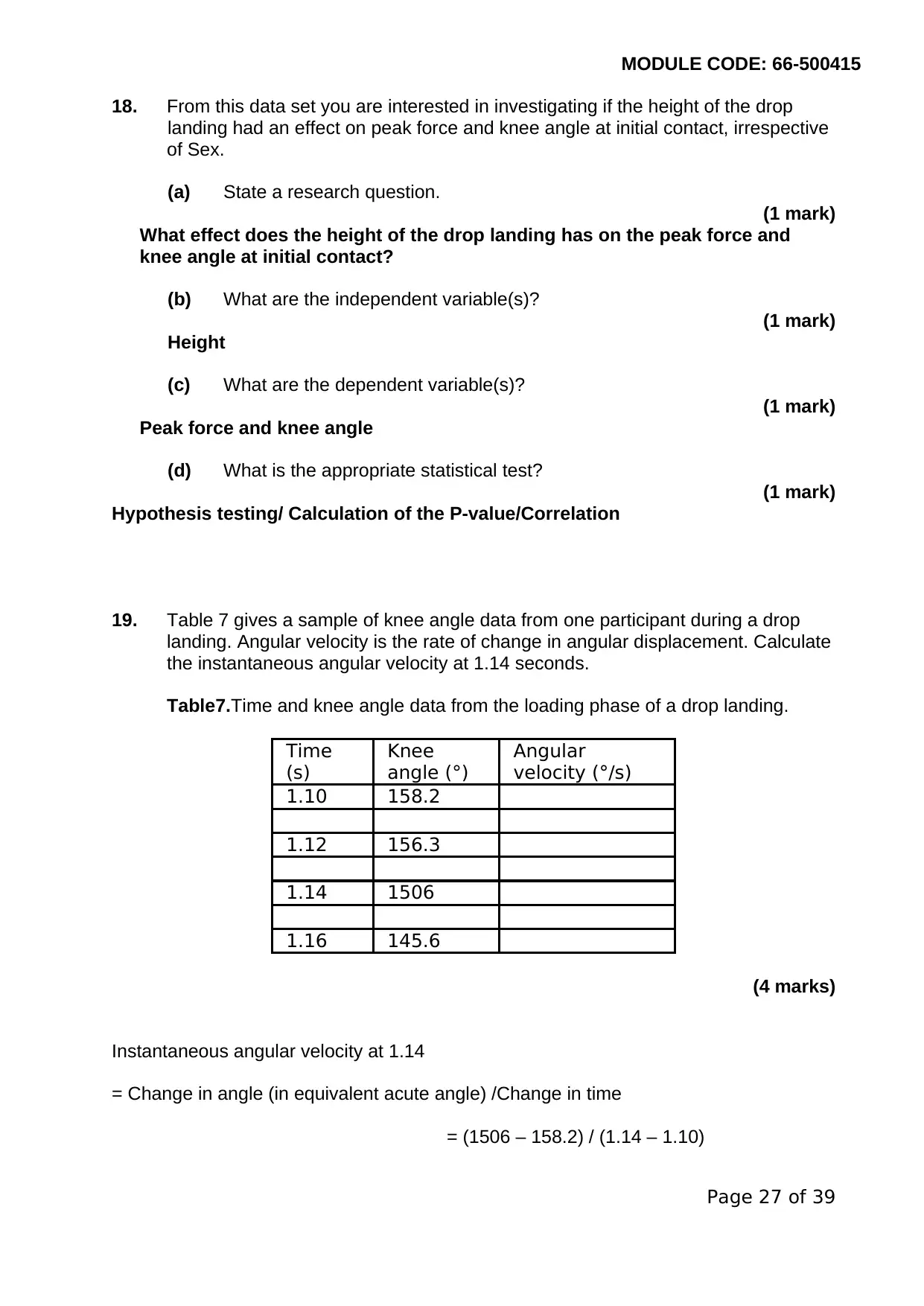
18. From this data set you are interested in investigating if the height of the drop
landing had an effect on peak force and knee angle at initial contact, irrespective
of Sex.
(a) State a research question.
(1 mark)
What effect does the height of the drop landing has on the peak force and
knee angle at initial contact?
(b) What are the independent variable(s)?
(1 mark)
Height
(c) What are the dependent variable(s)?
(1 mark)
Peak force and knee angle
(d) What is the appropriate statistical test?
(1 mark)
Hypothesis testing/ Calculation of the P-value/Correlation
19. Table 7 gives a sample of knee angle data from one participant during a drop
landing. Angular velocity is the rate of change in angular displacement. Calculate
the instantaneous angular velocity at 1.14 seconds.
Table7.Time and knee angle data from the loading phase of a drop landing.
Time
(s)
Knee
angle (°)
Angular
velocity (°/s)
1.10 158.2
1.12 156.3
1.14 1506
1.16 145.6
(4 marks)
Instantaneous angular velocity at 1.14
= Change in angle (in equivalent acute angle) /Change in time
= (1506 – 158.2) / (1.14 – 1.10)
Page 27 of 39

MODULE CODE: 66-500415
= 5200m/s
Page 28 of 39
= 5200m/s
Page 28 of 39
Secure Best Marks with AI Grader
Need help grading? Try our AI Grader for instant feedback on your assignments.
MODULE CODE: 66-500415
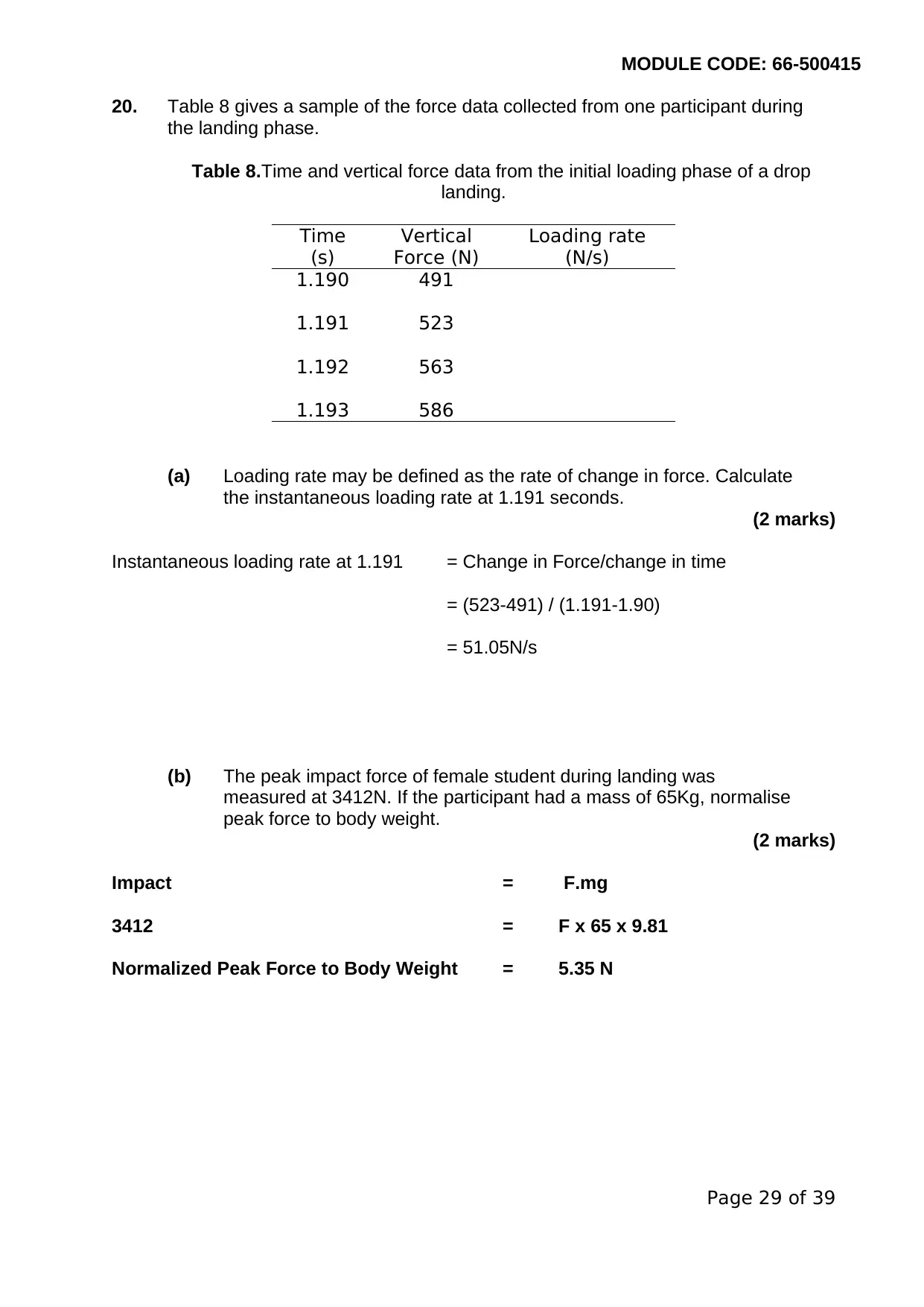
20. Table 8 gives a sample of the force data collected from one participant during
the landing phase.
Table 8.Time and vertical force data from the initial loading phase of a drop
landing.
Time
(s)
Vertical
Force (N)
Loading rate
(N/s)
1.190 491
1.191 523
1.192 563
1.193 586
(a) Loading rate may be defined as the rate of change in force. Calculate
the instantaneous loading rate at 1.191 seconds.
(2 marks)
Instantaneous loading rate at 1.191 = Change in Force/change in time
= (523-491) / (1.191-1.90)
= 51.05N/s
(b) The peak impact force of female student during landing was
measured at 3412N. If the participant had a mass of 65Kg, normalise
peak force to body weight.
(2 marks)
Impact = F.mg
3412 = F x 65 x 9.81
Normalized Peak Force to Body Weight = 5.35 N
Page 29 of 39

MODULE CODE: 66-500415
Page 30 of 39
Page 30 of 39
MODULE CODE: 66-500415
21. As a follow up study you are interested in the difference in kinetic and kinematic
variables between males and females when landing a drop jump from two
different heights. Based on the collected data set, a mixed ANOVA (2 groups x 2
heights) was used to analyse the data. The tables in Appendix 1 shows the
SPSS output for this analysis carried out for two variables: Peak force (BW) and
Peak knee angle (°).
(a) Based on this analysis output, you should write a 250 word (maximum)
abstract for this study. Your abstract should address the main areas of
background, aim, methods, results, conclusions, implications.
(10 marks)
Drops jumps are often part of the exercises used to train in lowering body power
to improve performance in jumping. However, there is little knowledge on how
kinematics and kinetics vary between men and women. Therefore, this study
sought to investigate the difference in kinetic and kinematic variables between
males and females when landing a drop jump from two different heights. 39
(N=39) participants were recruited for the study, for which, 18 were female, and 21
were male. The experiment was conducted for the male gender and the the
kinetics and kinematics results recorded in table form. The experiment was also
conducted for the female gender and the results recorded. The variables for the
experiment were Peak force Low Heigh Bw, Peak Force High Height BW, Peak
Knee Angle Low, and Peak knee Angle High. The data collected was analyzed
using a mixed ANOVA (2 groups x 2 heights). Findings from the study showed
that there was a significance difference in the kinematic and kinetic variables
between males and females when landing a drop jump from two different heights.
The results suggest that females are more likely to the affected by the landing
than males.
Page 31 of 39
Paraphrase This Document
Need a fresh take? Get an instant paraphrase of this document with our AI Paraphraser

MODULE CODE: 66-500415
Question 21 continues on the next page
Page 32 of 39
Question 21 continues on the next page
Page 32 of 39

MODULE CODE: 66-500415
(b) Highlight some of the key limitations with the data collection and
processing of the outlined study.
(5marks)
Some of the key limitations with the data collected and processing include: The
data considered a specific group of people and therefore cannot be generalized
for all cases; Only one statistical technique was used to analyse the data and this
affects validity; and the number of participants was relatively low to study the
variables.
Page 33 of 39
MODULE CODE: 66-500415
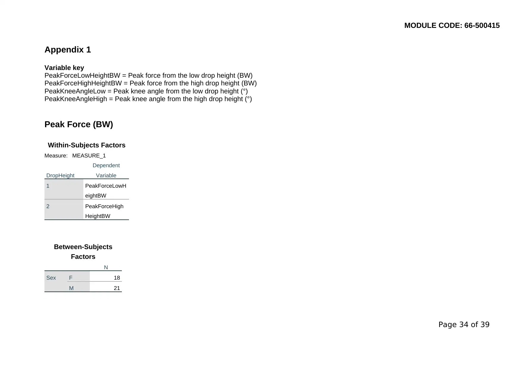
Appendix 1
Variable key
PeakForceLowHeightBW = Peak force from the low drop height (BW)
PeakForceHighHeightBW = Peak force from the high drop height (BW)
PeakKneeAngleLow = Peak knee angle from the low drop height (°)
PeakKneeAngleHigh = Peak knee angle from the high drop height (°)
Peak Force (BW)
Within-Subjects Factors
Measure: MEASURE_1
DropHeight
Dependent
Variable
1 PeakForceLowH
eightBW
2 PeakForceHigh
HeightBW
Between-Subjects
Factors
N
Sex F 18
M 21
Page 34 of 39
Secure Best Marks with AI Grader
Need help grading? Try our AI Grader for instant feedback on your assignments.
MODULE CODE: 66-500415
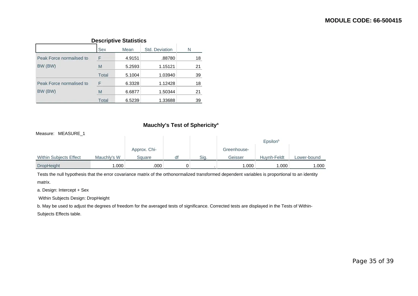
Descriptive Statistics
Sex Mean Std. Deviation N
Peak Force normailsed to
BW (BW)
F 4.9151 .88780 18
M 5.2593 1.15121 21
Total 5.1004 1.03940 39
Peak Force normalised to
BW (BW)
F 6.3328 1.12428 18
M 6.6877 1.50344 21
Total 6.5239 1.33688 39
Mauchly's Test of Sphericitya
Measure: MEASURE_1
Within Subjects Effect Mauchly's W
Approx. Chi-
Square df Sig.
Epsilonb
Greenhouse-
Geisser Huynh-Feldt Lower-bound
DropHeight 1.000 .000 0 . 1.000 1.000 1.000
Tests the null hypothesis that the error covariance matrix of the orthonormalized transformed dependent variables is proportional to an identity
matrix.
a. Design: Intercept + Sex
Within Subjects Design: DropHeight
b. May be used to adjust the degrees of freedom for the averaged tests of significance. Corrected tests are displayed in the Tests of Within-
Subjects Effects table.
Page 35 of 39
MODULE CODE: 66-500415
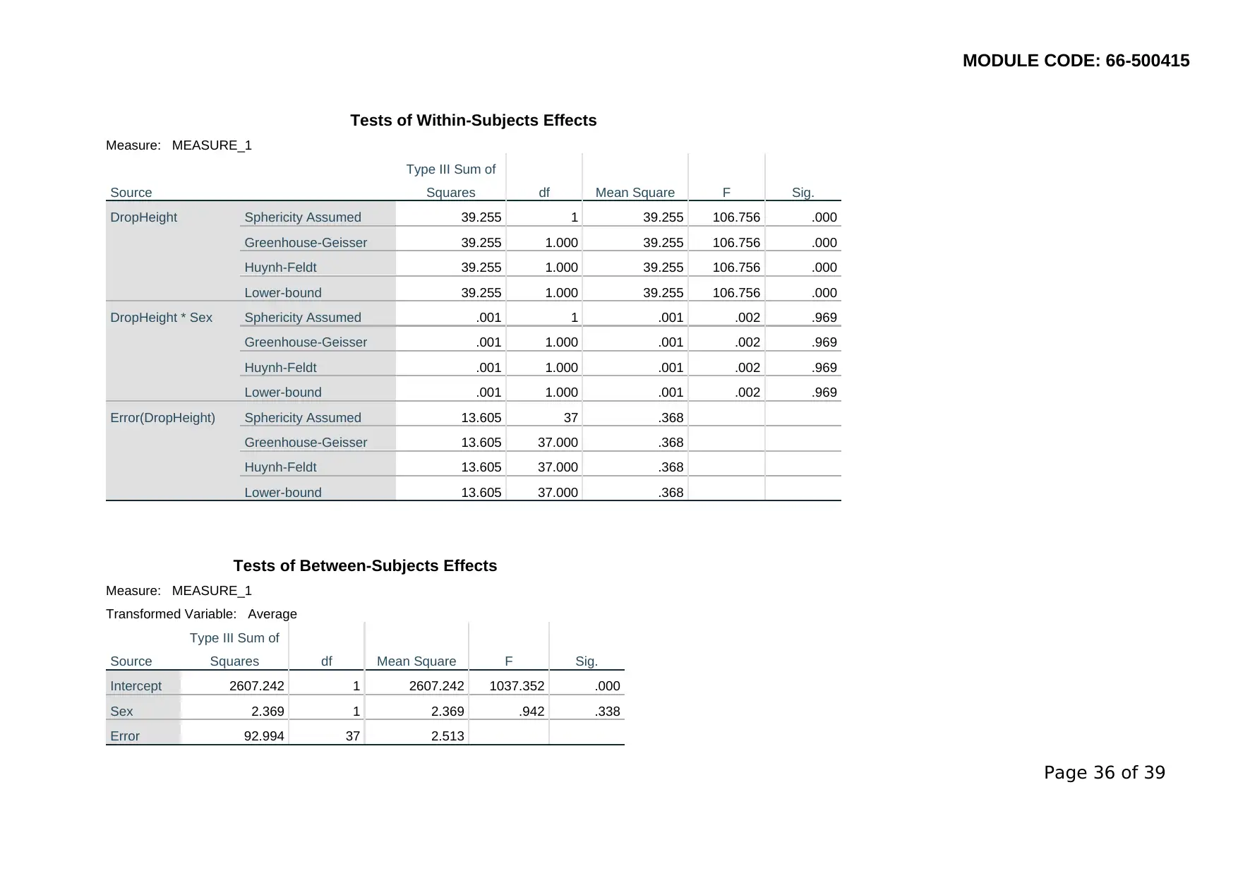
Tests of Within-Subjects Effects
Measure: MEASURE_1
Source
Type III Sum of
Squares df Mean Square F Sig.
DropHeight Sphericity Assumed 39.255 1 39.255 106.756 .000
Greenhouse-Geisser 39.255 1.000 39.255 106.756 .000
Huynh-Feldt 39.255 1.000 39.255 106.756 .000
Lower-bound 39.255 1.000 39.255 106.756 .000
DropHeight * Sex Sphericity Assumed .001 1 .001 .002 .969
Greenhouse-Geisser .001 1.000 .001 .002 .969
Huynh-Feldt .001 1.000 .001 .002 .969
Lower-bound .001 1.000 .001 .002 .969
Error(DropHeight) Sphericity Assumed 13.605 37 .368
Greenhouse-Geisser 13.605 37.000 .368
Huynh-Feldt 13.605 37.000 .368
Lower-bound 13.605 37.000 .368
Tests of Between-Subjects Effects
Measure: MEASURE_1
Transformed Variable: Average
Source
Type III Sum of
Squares df Mean Square F Sig.
Intercept 2607.242 1 2607.242 1037.352 .000
Sex 2.369 1 2.369 .942 .338
Error 92.994 37 2.513
Page 36 of 39

MODULE CODE: 66-500415
Peak knee angle (°)
Within-Subjects Factors
Measure: MEASURE_1
DropHeight
Dependent
Variable
1 PeakKneeAngle
LowHeightdegre
es
2 PeakAnkleAngle
HighHeightdegre
es
Between-Subjects
Factors
N
Sex F 18
M 21
Page 37 of 39
Peak knee angle (°)
Within-Subjects Factors
Measure: MEASURE_1
DropHeight
Dependent
Variable
1 PeakKneeAngle
LowHeightdegre
es
2 PeakAnkleAngle
HighHeightdegre
es
Between-Subjects
Factors
N
Sex F 18
M 21
Page 37 of 39
Paraphrase This Document
Need a fresh take? Get an instant paraphrase of this document with our AI Paraphraser
MODULE CODE: 66-500415
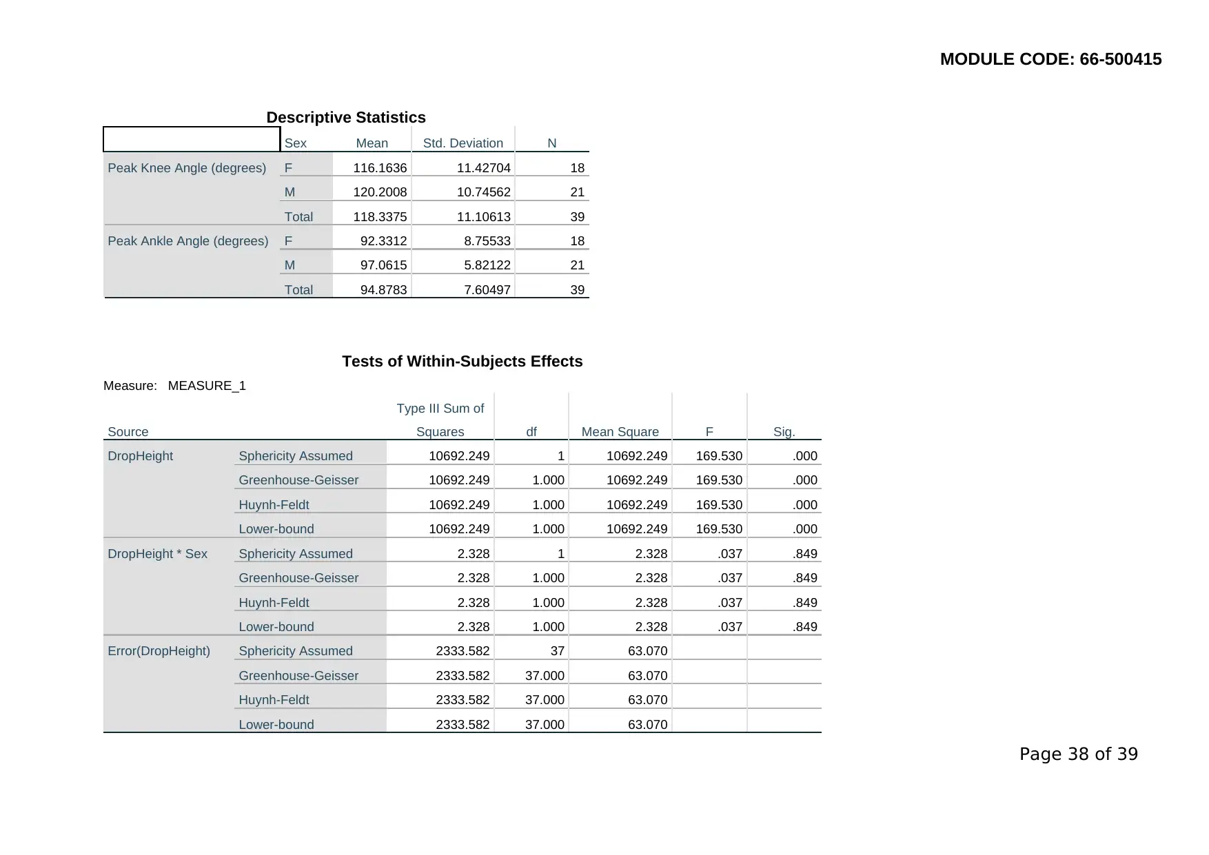
Descriptive Statistics
Sex Mean Std. Deviation N
Peak Knee Angle (degrees) F 116.1636 11.42704 18
M 120.2008 10.74562 21
Total 118.3375 11.10613 39
Peak Ankle Angle (degrees) F 92.3312 8.75533 18
M 97.0615 5.82122 21
Total 94.8783 7.60497 39
Tests of Within-Subjects Effects
Measure: MEASURE_1
Source
Type III Sum of
Squares df Mean Square F Sig.
DropHeight Sphericity Assumed 10692.249 1 10692.249 169.530 .000
Greenhouse-Geisser 10692.249 1.000 10692.249 169.530 .000
Huynh-Feldt 10692.249 1.000 10692.249 169.530 .000
Lower-bound 10692.249 1.000 10692.249 169.530 .000
DropHeight * Sex Sphericity Assumed 2.328 1 2.328 .037 .849
Greenhouse-Geisser 2.328 1.000 2.328 .037 .849
Huynh-Feldt 2.328 1.000 2.328 .037 .849
Lower-bound 2.328 1.000 2.328 .037 .849
Error(DropHeight) Sphericity Assumed 2333.582 37 63.070
Greenhouse-Geisser 2333.582 37.000 63.070
Huynh-Feldt 2333.582 37.000 63.070
Lower-bound 2333.582 37.000 63.070
Page 38 of 39
MODULE CODE: 66-500415
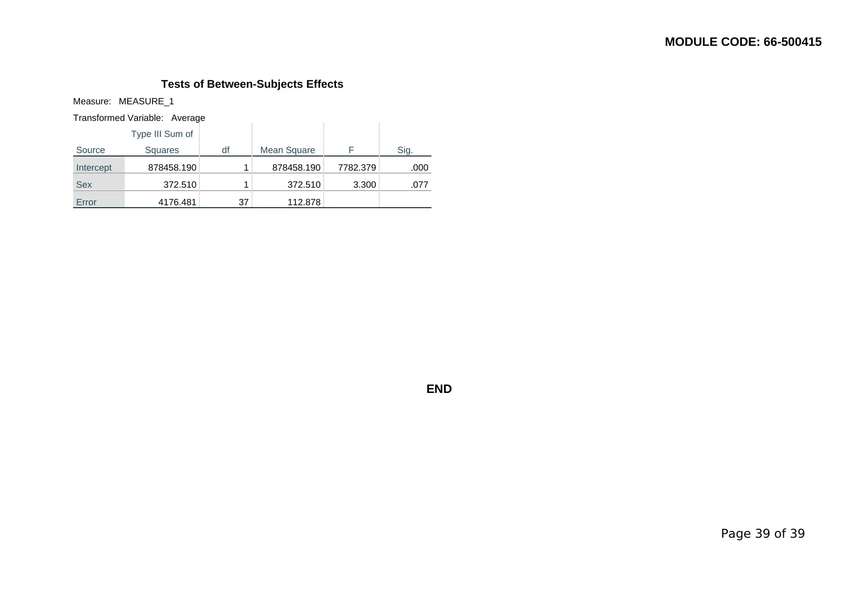
Tests of Between-Subjects Effects
Measure: MEASURE_1
Transformed Variable: Average
Source
Type III Sum of
Squares df Mean Square F Sig.
Intercept 878458.190 1 878458.190 7782.379 .000
Sex 372.510 1 372.510 3.300 .077
Error 4176.481 37 112.878
END
Page 39 of 39
Tests of Between-Subjects Effects
Measure: MEASURE_1
Transformed Variable: Average
Source
Type III Sum of
Squares df Mean Square F Sig.
Intercept 878458.190 1 878458.190 7782.379 .000
Sex 372.510 1 372.510 3.300 .077
Error 4176.481 37 112.878
END
Page 39 of 39
1 out of 39
Related Documents

Your All-in-One AI-Powered Toolkit for Academic Success.
+13062052269
info@desklib.com
Available 24*7 on WhatsApp / Email
![[object Object]](/_next/static/media/star-bottom.7253800d.svg)
Unlock your academic potential
© 2024 | Zucol Services PVT LTD | All rights reserved.