CN5002 Advanced Reaction Engineering: Benzene Gas Diffusion Simulation

This report details a molecular dynamics simulation of benzene gas, conducted using the ASE package in Google Colab. The assignment aimed to determine the diffusion coefficient (D) of benzene gas at 500K and investigate the impact of temperature and timestep variations on the D value. The methodology involved designing a benzene gas model, setting computational parameters, running the simulation, calculating atomic displacements, and determining the D value using linear regression. The simulation was run under three different scenarios with varying temperatures and timesteps. The results showed the calculated D value and its comparison with theoretical values from external sources. The report includes detailed methodology, results, and discussion, providing insights into the factors affecting gas diffusion in the context of benzene gas.

National University of Singapore (NUS)
Department of Chemical & Biomolecular Engineering
CN5002: Advanced Reaction Engineering
Master of Science in Chemical Engineering
AY 2020/2021 Semester 2
Week 2 Homework Assignment 1 Written Report
Title: Molecular Dynamic Simulation of Benzene Gas
Student Name: Abdul Hannan Bin Abdul Rahman
Student Number: A0229546W
Lecturer Name: Assistant Professor Sergey Kozlov

ageP 1 of 8
Abstract
In this assignment, the molecular dynamic simulation of benzene gas molecule was performed
initially at 500K. The gas molecule was simulated using the atomic simulation environment
(ASE) package in Google Colab notebook, involving the use of Python codings. The aim of
this assignment is to determine the value of diffusion coefficient (D) of benzene gas at 500K
using linear regression function after calculating both the magnitude of atomic displacements
and the total elapsed time from the result of this simulation. In addition to that, the simulation
was also run few several times at different system temperature and timestep value for different
scenarios to investigate the effect of these two parameters on value of gas diffusion coefficient.
While working on this assignment, different functions and methods from the ASE modules, in
addition to a square atomic displacement formula, as well as ASE unit conversion factors, were
all used in order to obtain the final calculated value of diffusion coefficient (D) of benzene gas.
The calculated D value will then later be analysed and compared with the expected theoretical
D value from that of external sources in the discussion section of this written report.
1. Aims and Objectives
Aims: To determine the value of diffusion coefficient (D) of benzene gas at initial 500 K and
to investigate the effect of temperature and timestep on D value for different scenarios.
Objectives:
▪ Simple model of benzene gas structure will be designed with specified sizes and
dimensions using the ‘molecule’ function from ase.build module.
▪ Initial atomic position of benzene gas molecule at thermodynamic equilibrium system
will be calculated in different directions using the gas.get positon method.
▪ Magnitude of the atomic displacements will be recorded using the ‘norm’ function
from numpy.linalg module.
▪ Total elapsed time required to run the entire molecular dynamic simulation will be
recorded using the gas.get_time method.
▪ Diffusion coefficient (D) of benzene gas will be calculated from the slope of plotted
graph of atomic displacement over time using linear regression function.

ageP 2 of 8
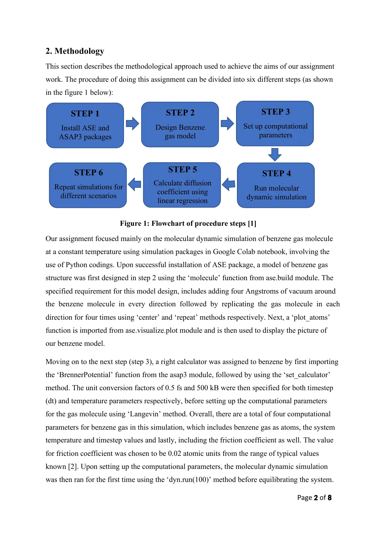
2. Methodology
This section describes the methodological approach used to achieve the aims of our assignment
work. The procedure of doing this assignment can be divided into six different steps (as shown
in the figure 1 below):
Figure 1: Flowchart of procedure steps [1]
Our assignment focused mainly on the molecular dynamic simulation of benzene gas molecule
at a constant temperature using simulation packages in Google Colab notebook, involving the
use of Python codings. Upon successful installation of ASE package, a model of benzene gas
structure was first designed in step 2 using the ‘molecule’ function from ase.build module. The
specified requirement for this model design, includes adding four Angstroms of vacuum around
the benzene molecule in every direction followed by replicating the gas molecule in each
direction for four times using ‘center’ and ‘repeat’ methods respectively. Next, a ‘plot_atoms’
function is imported from ase.visualize.plot module and is then used to display the picture of
our benzene model.
Moving on to the next step (step 3), a right calculator was assigned to benzene by first importing
the ‘BrennerPotential’ function from the asap3 module, followed by using the ‘set_calculator’
method. The unit conversion factors of 0.5 fs and 500 kB were then specified for both timestep
(dt) and temperature parameters respectively, before setting up the computational parameters
for the gas molecule using ‘Langevin’ method. Overall, there are a total of four computational
parameters for benzene gas in this simulation, which includes benzene gas as atoms, the system
temperature and timestep values and lastly, including the friction coefficient as well. The value
for friction coefficient was chosen to be 0.02 atomic units from the range of typical values
known [2]. Upon setting up the computational parameters, the molecular dynamic simulation
was then ran for the first time using the ‘dyn.run(100)’ method before equilibrating the system.
STEP 1
Install ASE and
ASAP3 packages
STEP 2
Design Benzene
gas model
STEP 3
Set up computational
parameters
STEP 4
Run molecular
dynamic simulation
STEP 5
Calculate diffusion
coefficient using
linear regression
STEP 6
Repeat simulations for
different scenarios

age ofP 3 8
The maximum number of steps was selected to be 100 (50 fs timestep value) to ensure a quick
simulation process while performing iterative calculation for loop later on. In step 4, the initial
atomic position of the gas molecule was first calculated using the get_positions method. Upon
calculating the initial position, the value of atomic displacement was then iteratively calculated
using a loop at the same maximum number of 100 steps and fixed system temperature of 500
K. The total number of atoms for the benzene gas model was calculated to be at around 768
atoms using the get_global_number_of_atoms method. Similarly, the value of iteration (i) was
chosen to be at 768 as equal as the total number of gas atoms. The Python coding used for this
iterative calculation can be found in our submitted ‘simulation code.py’ file. Afterwards, the
magnitude of atomic displacements and the elapsed time for simulation were then recorded
using both the imported ‘norm’ function from the numpy.linalg module and the ‘dyn.get_time’
method respectively.
Upon recording both the atomic displacement magnitude and total elapsed time for simulation,
the value of diffusion coefficient (D) for benzene gas was then calculated in step 5 at initial
constant temperature of 500 K. This can be done by converting the square atomic displacement
formula (equation 1 below) into linear equation (y = mx + c), where y is the value of atomic
displacement and x is the total elapsed time.
Equation 1: Square Atomic Displacement Formula [1]
The slope of the plotted graph of value of atomic displacement over total elapsed time will give
us value of (6.D.Nat), where Nat is equal to 768 as total number of atoms in benzene molecule.
The value of D can then be calculated from the value of slope obtained from plotting the graph.
To plot the graph, quantitative sets of both x and y data need to be specified in the code cell of
Google Colab notebook, using values atomic displacement magnitude and total elapsed time
recorded earlier. Next, ‘linregress’ function from scripy.stats module and ‘plt’ function from
Matplotlib.pyplt module would then be used to plot the graph before the slope value can be
determined to calculate D. Theoretically, we would expect a single linear graph when executing
both functions for our sets of x and y data [3]. The Python coding used for plotting this linear
graph can be found in our submitted ‘simulation code.py’ file. Moving on to the next step (step
6), the molecular dynamic simulation was also run few times using different temperature and
timestep value for different scenarios to investigate the effect of these two parameters on value
of gas diffusion coefficient (D). In total, there are three scenarios in this assignment work. The

ageP 4 of 8
values of computational parameters (temperature and timestep) used for these scenarios are
shown in table 1 below. Note that the friction coefficient, iteration (i) value and maximum
number of steps while running the simulation were all kept constant for all 3 different scenarios
at 0.02, 768 and 100 respectively.
Temperature (Kelvin) Timestep (femtosecond)
Scenario 1 500 0.50
Scenario 2 300 1.00
Scenario 3 700 0.25
Table 1: Values of computational parameters used for 3 different scenarios
The results of simulating benzene gas molecule for all 3 scenarios were all obtained in the form
of quantitative data of the atomic displacement and total elapsed time. The data will then be
imported from our ‘w2_homework[1]_5020.ipynb’ file into an Excel spreadsheet file, followed
by plotting linear graphs of these data for all three scenarios. We can then perform data analysis
by observing these plotted graphs for each scenario and from this analysis, this would allow us
to examine the effect of altering these two parameters on the D value of benzene gas and make
final deduction remarks from these results.
3. Results and Discussion
The results of our assignment work are presented and discussed in this section. The following
figures below are obtained from our Google Colab notebook:
Figure 2: Atomic structure of Figure 3: Plotted graph of atomic displacement
benzene gas model over time at 500 K (scenario 1)

age ofP 5 8
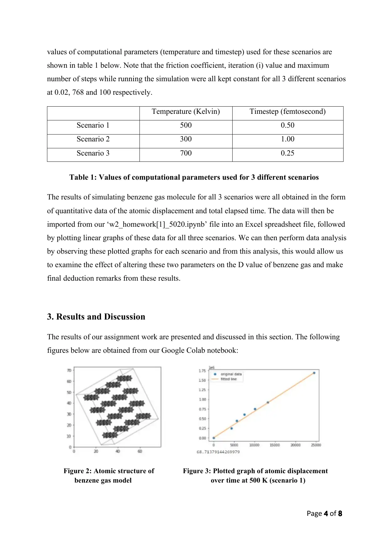
Figure 2 shows the picture of the atomic structure of our benzene gas molecule obtained in step
2 at rotation of ‘10x,20y,30z’. For each benzene gas molecule, there are 12 atoms in total (6
atoms of carbon and 6 atoms of hydrogen). Upon replicating the benzene gas molecule four
times in each direction of x, y and z, we would have around 64 molecules of benzene gas. Thus,
the total number of atoms (Nat) for our gas model would be around 768 atoms.
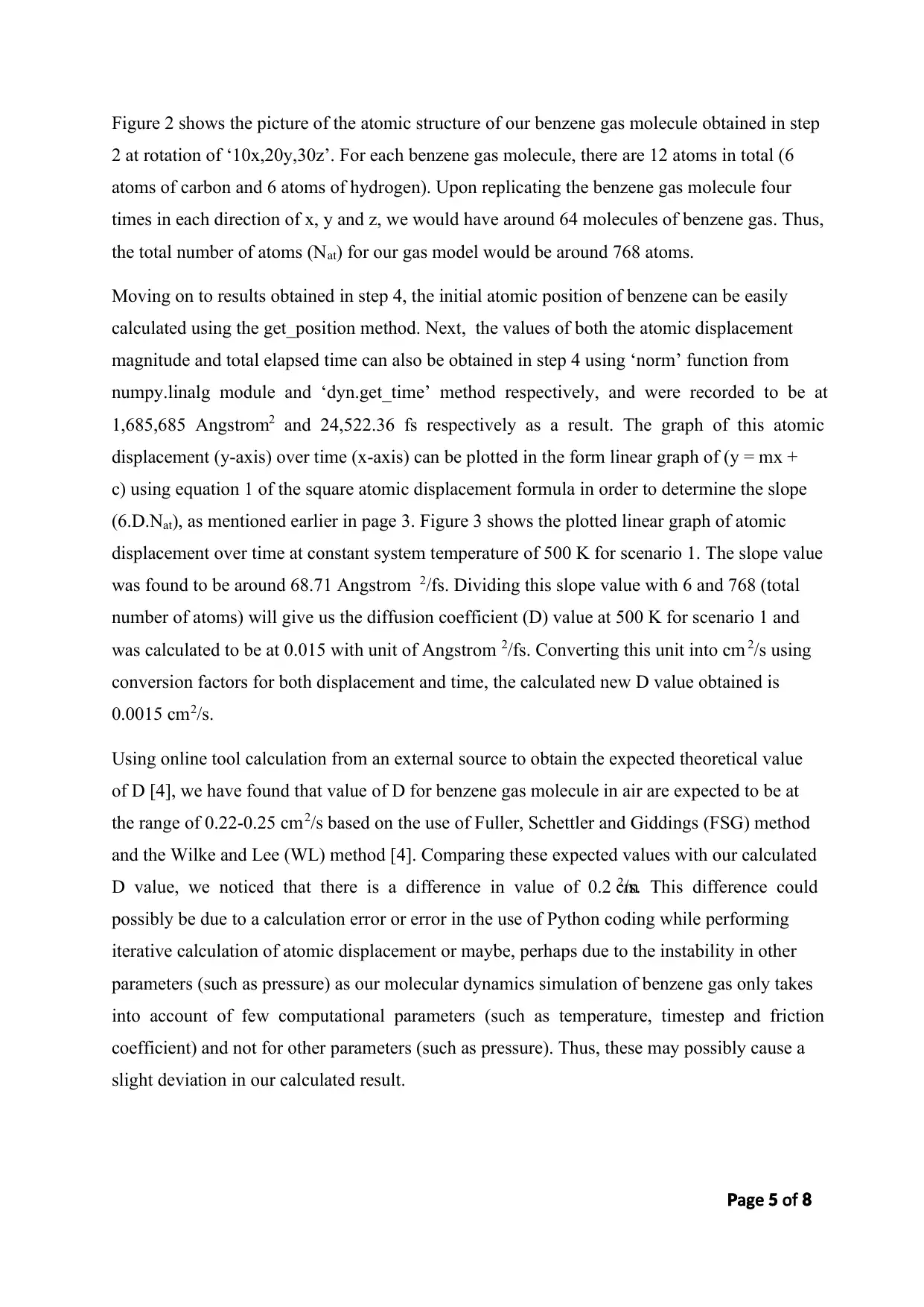
Moving on to results obtained in step 4, the initial atomic position of benzene can be easily
calculated using the get_position method. Next, the values of both the atomic displacement
magnitude and total elapsed time can also be obtained in step 4 using ‘norm’ function from
numpy.linalg module and ‘dyn.get_time’ method respectively, and were recorded to be at
1,685,685 Angstrom2 and 24,522.36 fs respectively as a result. The graph of this atomic
displacement (y-axis) over time (x-axis) can be plotted in the form linear graph of (y = mx +
c) using equation 1 of the square atomic displacement formula in order to determine the slope
(6.D.Nat), as mentioned earlier in page 3. Figure 3 shows the plotted linear graph of atomic
displacement over time at constant system temperature of 500 K for scenario 1. The slope value
was found to be around 68.71 Angstrom 2/fs. Dividing this slope value with 6 and 768 (total
number of atoms) will give us the diffusion coefficient (D) value at 500 K for scenario 1 and
was calculated to be at 0.015 with unit of Angstrom 2/fs. Converting this unit into cm 2/s using
conversion factors for both displacement and time, the calculated new D value obtained is
0.0015 cm2/s.
Using online tool calculation from an external source to obtain the expected theoretical value
of D [4], we have found that value of D for benzene gas molecule in air are expected to be at
the range of 0.22-0.25 cm2/s based on the use of Fuller, Schettler and Giddings (FSG) method
and the Wilke and Lee (WL) method [4]. Comparing these expected values with our calculated
D value, we noticed that there is a difference in value of 0.2 cm2/s. This difference could
possibly be due to a calculation error or error in the use of Python coding while performing
iterative calculation of atomic displacement or maybe, perhaps due to the instability in other
parameters (such as pressure) as our molecular dynamics simulation of benzene gas only takes
into account of few computational parameters (such as temperature, timestep and friction
coefficient) and not for other parameters (such as pressure). Thus, these may possibly cause a
slight deviation in our calculated result.

ageP 6 of 8
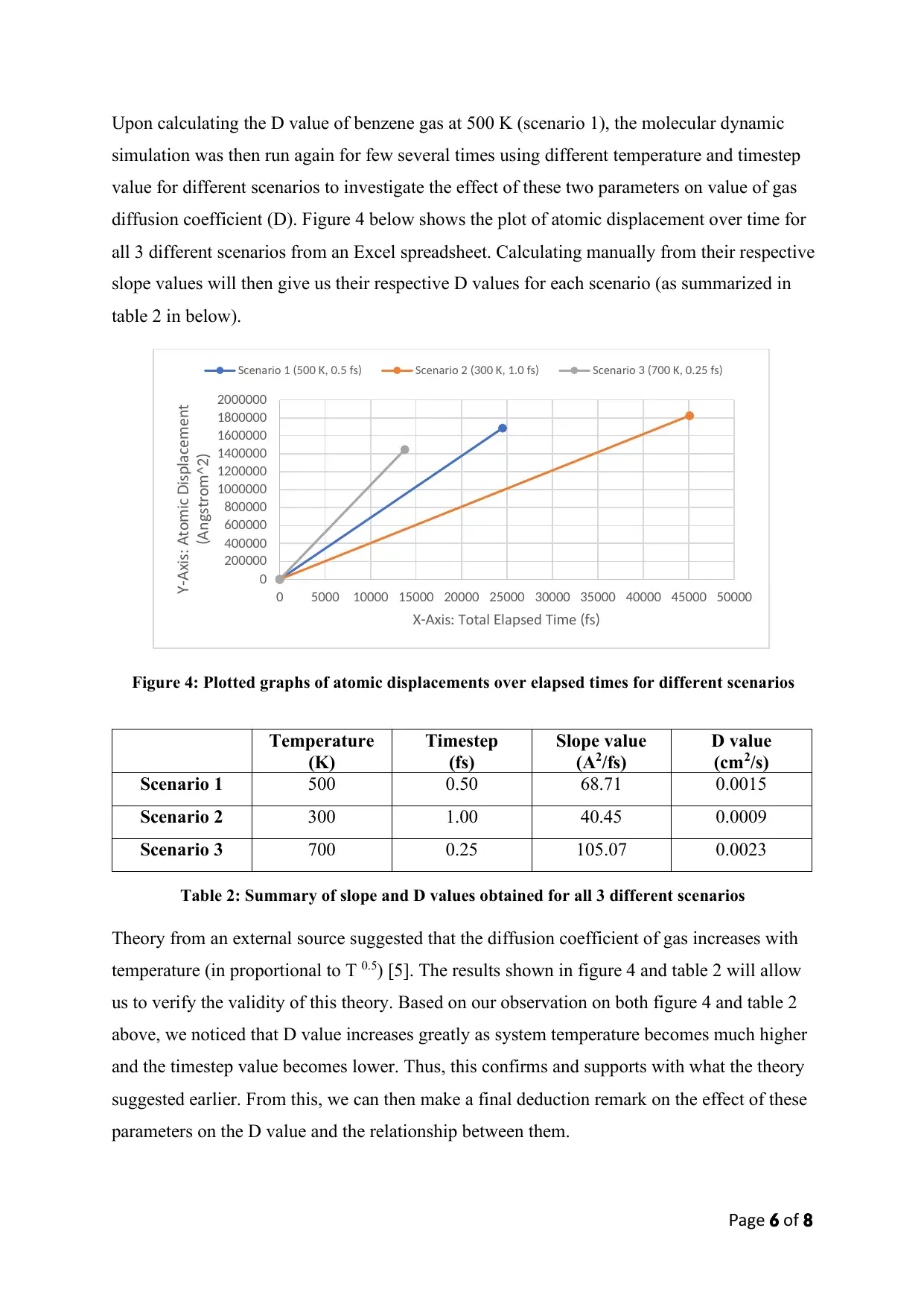
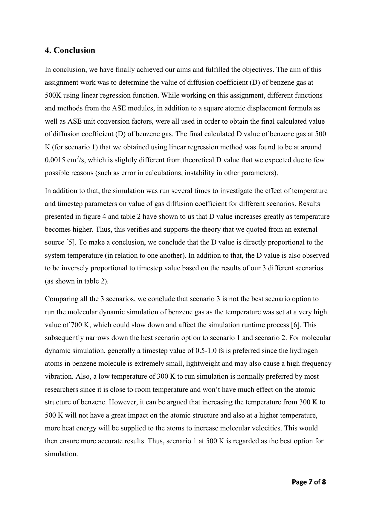
Upon calculating the D value of benzene gas at 500 K (scenario 1), the molecular dynamic
simulation was then run again for few several times using different temperature and timestep
value for different scenarios to investigate the effect of these two parameters on value of gas
diffusion coefficient (D). Figure 4 below shows the plot of atomic displacement over time for
all 3 different scenarios from an Excel spreadsheet. Calculating manually from their respective
slope values will then give us their respective D values for each scenario (as summarized in
table 2 in below).
Figure 4: Plotted graphs of atomic displacements over elapsed times for different scenarios
Temperature
(K)
Timestep
(fs)
Slope value
(A2/fs)
D value
(cm2/s)
Scenario 1 500 0.50 68.71 0.0015
Scenario 2 300 1.00 40.45 0.0009
Scenario 3 700 0.25 105.07 0.0023
Table 2: Summary of slope and D values obtained for all 3 different scenarios
Theory from an external source suggested that the diffusion coefficient of gas increases with
temperature (in proportional to T 0.5) [5]. The results shown in figure 4 and table 2 will allow
us to verify the validity of this theory. Based on our observation on both figure 4 and table 2
above, we noticed that D value increases greatly as system temperature becomes much higher
and the timestep value becomes lower. Thus, this confirms and supports with what the theory
suggested earlier. From this, we can then make a final deduction remark on the effect of these
parameters on the D value and the relationship between them.
0
200000
400000
600000
800000
1000000
1200000
1400000
1600000
1800000
2000000
0 5000 10000 15000 20000 25000 30000 35000 40000 45000 50000
is to i is la e entY-Ax : A m c D p c m
ngstro(A m^2)
is Total la sed Ti e fsX-Ax : E p m ( )
enario fsSc 1 (500 K, 0.5 ) enario fsSc 2 (300 K, 1.0 ) enario fsSc 3 (700 K, 0.25 )

age ofP 7 8
4. Conclusion
In conclusion, we have finally achieved our aims and fulfilled the objectives. The aim of this
assignment work was to determine the value of diffusion coefficient (D) of benzene gas at
500K using linear regression function. While working on this assignment, different functions
and methods from the ASE modules, in addition to a square atomic displacement formula as
well as ASE unit conversion factors, were all used in order to obtain the final calculated value
of diffusion coefficient (D) of benzene gas. The final calculated D value of benzene gas at 500
K (for scenario 1) that we obtained using linear regression method was found to be at around
0.0015 cm2/s, which is slightly different from theoretical D value that we expected due to few
possible reasons (such as error in calculations, instability in other parameters).
In addition to that, the simulation was run several times to investigate the effect of temperature
and timestep parameters on value of gas diffusion coefficient for different scenarios. Results
presented in figure 4 and table 2 have shown to us that D value increases greatly as temperature
becomes higher. Thus, this verifies and supports the theory that we quoted from an external
source [5]. To make a conclusion, we conclude that the D value is directly proportional to the
system temperature (in relation to one another). In addition to that, the D value is also observed
to be inversely proportional to timestep value based on the results of our 3 different scenarios
(as shown in table 2).
Comparing all the 3 scenarios, we conclude that scenario 3 is not the best scenario option to
run the molecular dynamic simulation of benzene gas as the temperature was set at a very high
value of 700 K, which could slow down and affect the simulation runtime process [6]. This
subsequently narrows down the best scenario option to scenario 1 and scenario 2. For molecular
dynamic simulation, generally a timestep value of 0.5-1.0 fs is preferred since the hydrogen
atoms in benzene molecule is extremely small, lightweight and may also cause a high frequency
vibration. Also, a low temperature of 300 K to run simulation is normally preferred by most
researchers since it is close to room temperature and won’t have much effect on the atomic
structure of benzene. However, it can be argued that increasing the temperature from 300 K to
500 K will not have a great impact on the atomic structure and also at a higher temperature,
more heat energy will be supplied to the atoms to increase molecular velocities. This would
then ensure more accurate results. Thus, scenario 1 at 500 K is regarded as the best option for
simulation.

ageP 8 of 8
References
1. https://colab.research.google.com/drive/1hdg9YvDqGVhdPBB25llbFBs7ECcckw9N
2. https://wiki.fysik.dtu.dk/ase/ase/md.html?highlight=friction
3. https://www.ncbi.nlm.nih.gov/pmc/articles/PMC3193570/ (see figure 2)
4. https://www3.epa.gov/ceampubl/learn2model/part-two/onsite/estdiffusion.html
5. https://chemeng.iisc.ac.in/kumaran/courses/chap2.pdf (see page 9)
6. https://www.hindawi.com/journals/isrn/2013/640125/