(PDF) Money and Banking : Assignment

Money and Banking
Name:
Institution:
9th May 2018

Q1:
This requires paying for the online cost. The cost is $249.
Check the appendix;
Q2:
a) Consider a portfolio that holds 60% of its capital in X and 40% in Y. What is the
distribution of the portfolio annual return?
Solution
The annual return of a portfolio is obtained based on the weight attached to the different
stocks under investigation. The following formula is applied to compute the annualized
return;
Portfolio annual rturn= ( wx∗μx ) + ( w y∗μ y )
Where,
wx=weight given¿ stock x
μx=average returns for stock x
w y=weight given¿ stock y
μy=average returns for stock y
From the information given, we have;
wx=60 %=0.6; μx=0.10; w y=4 0 %=0.6; μx=0.17

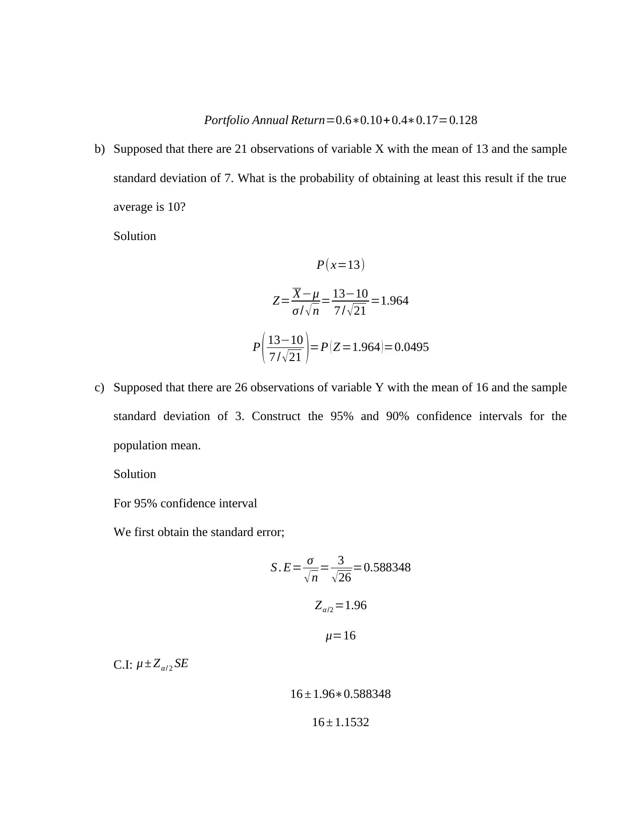
Portfolio Annual Return=0.6∗0.10+ 0.4∗0.17=0.128
b) Supposed that there are 21 observations of variable X with the mean of 13 and the sample
standard deviation of 7. What is the probability of obtaining at least this result if the true
average is 10?
Solution
P( x=13)
Z= X−μ
σ / √ n = 13−10
7 / √ 21 =1.964
P ( 13−10
7 / √21 )=P ( Z =1.964 )=0.0495
c) Supposed that there are 26 observations of variable Y with the mean of 16 and the sample
standard deviation of 3. Construct the 95% and 90% confidence intervals for the
population mean.
Solution
For 95% confidence interval
We first obtain the standard error;
S . E= σ
√n = 3
√26 =0.588348
Zα/2 =1.96
μ=16
C.I: μ ± Zα/ 2 SE
16 ± 1.96∗0.588348
16 ± 1.1532

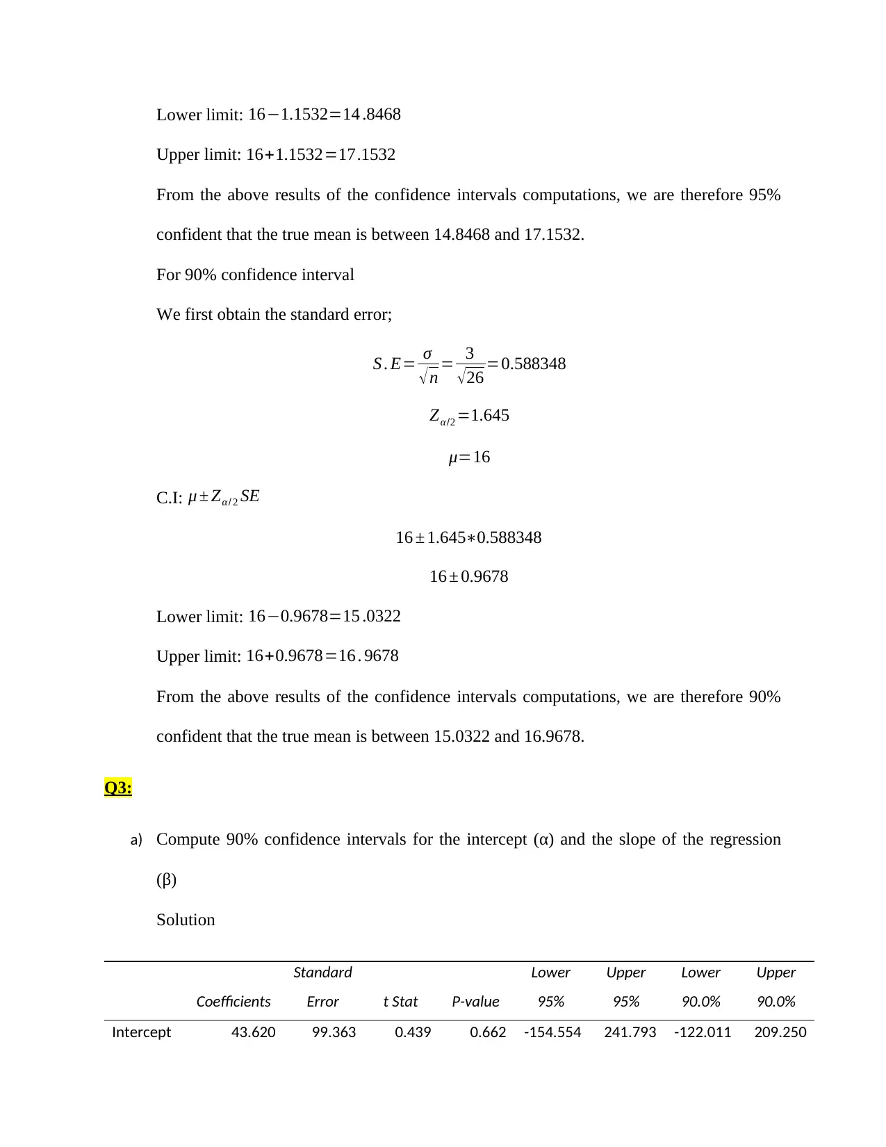
Lower limit: 16−1.1532=14 .8468
Upper limit: 16+1.1532=17.1532
From the above results of the confidence intervals computations, we are therefore 95%
confident that the true mean is between 14.8468 and 17.1532.
For 90% confidence interval
We first obtain the standard error;
S . E= σ
√n = 3
√26 =0.588348
Zα /2 =1.645
μ=16
C.I: μ ± Zα/ 2 SE
16 ± 1.645∗0.588348
16 ± 0.9678
Lower limit: 16−0.9678=15 .0322
Upper limit: 16+0.9678=16 . 9678
From the above results of the confidence intervals computations, we are therefore 90%
confident that the true mean is between 15.0322 and 16.9678.
Q3:
a) Compute 90% confidence intervals for the intercept (α) and the slope of the regression
(β)
Solution
Coefficients
Standard
Error t Stat P-value
Lower
95%
Upper
95%
Lower
90.0%
Upper
90.0%
Intercept 43.620 99.363 0.439 0.662 -154.554 241.793 -122.011 209.250

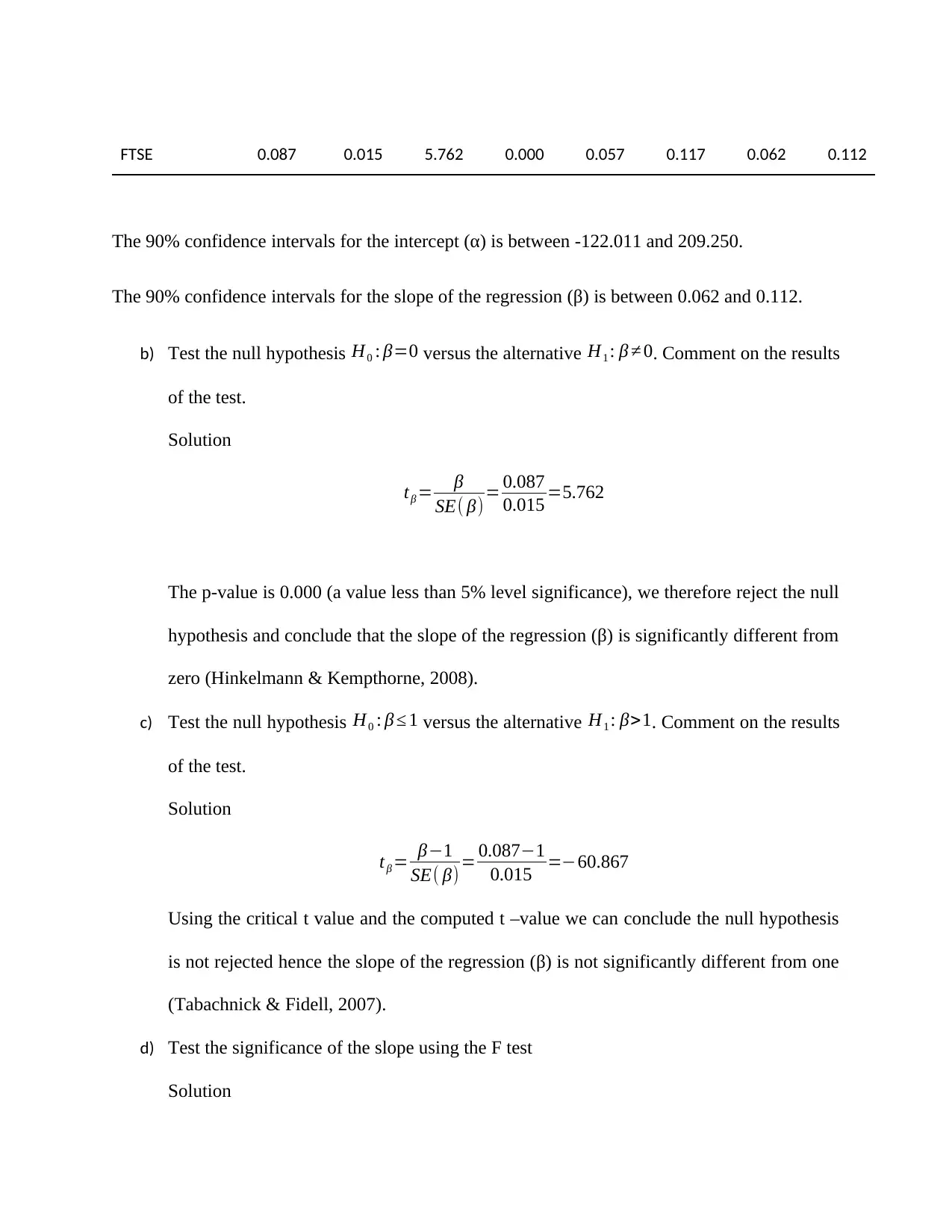
FTSE 0.087 0.015 5.762 0.000 0.057 0.117 0.062 0.112
The 90% confidence intervals for the intercept (α) is between -122.011 and 209.250.
The 90% confidence intervals for the slope of the regression (β) is between 0.062 and 0.112.
b) Test the null hypothesis H0 : β=0 versus the alternative H1 : β ≠ 0. Comment on the results
of the test.
Solution
tβ = β
SE( β)= 0.087
0.015 =5.762
The p-value is 0.000 (a value less than 5% level significance), we therefore reject the null
hypothesis and conclude that the slope of the regression (β) is significantly different from
zero (Hinkelmann & Kempthorne, 2008).
c) Test the null hypothesis H0 : β ≤ 1 versus the alternative H1 : β>1. Comment on the results
of the test.
Solution
tβ = β−1
SE( β) = 0.087−1
0.015 =−60.867
Using the critical t value and the computed t –value we can conclude the null hypothesis
is not rejected hence the slope of the regression (β) is not significantly different from one
(Tabachnick & Fidell, 2007).
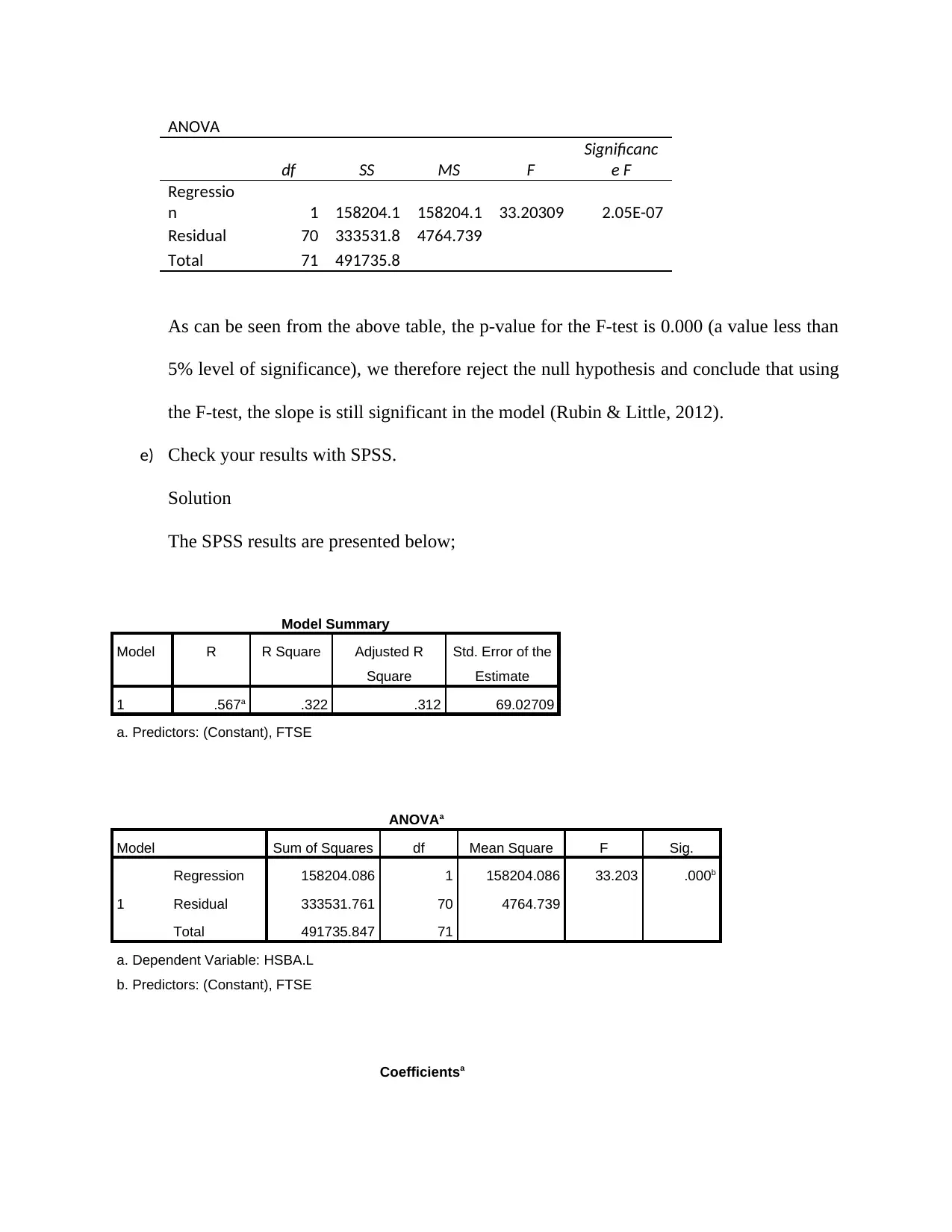
d) Test the significance of the slope using the F test
Solution

ANOVA
df SS MS F
Significanc
e F
Regressio
n 1 158204.1 158204.1 33.20309 2.05E-07
Residual 70 333531.8 4764.739
Total 71 491735.8
As can be seen from the above table, the p-value for the F-test is 0.000 (a value less than
5% level of significance), we therefore reject the null hypothesis and conclude that using
the F-test, the slope is still significant in the model (Rubin & Little, 2012).
e) Check your results with SPSS.
Solution
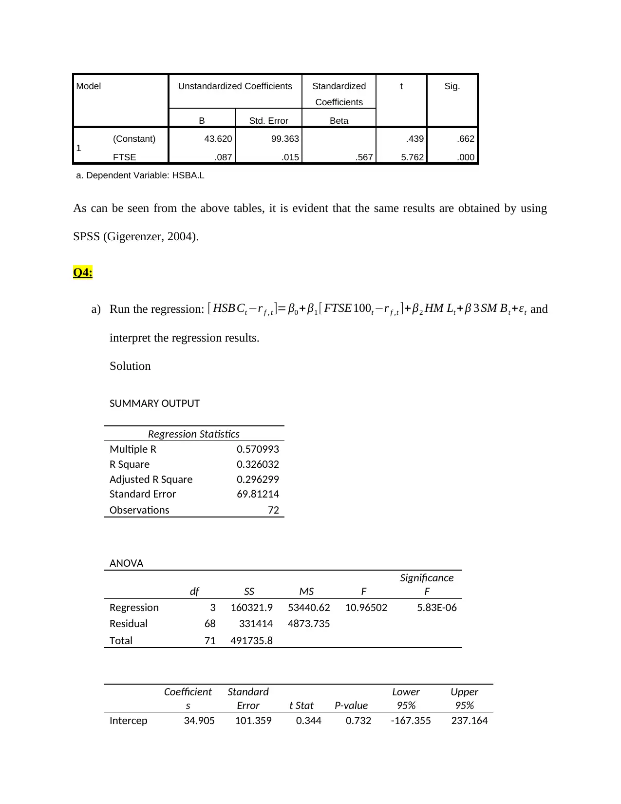
The SPSS results are presented below;
Model Summary
Model R R Square Adjusted R
Square
Std. Error of the
Estimate
1 .567a .322 .312 69.02709
a. Predictors: (Constant), FTSE
ANOVAa
Model Sum of Squares df Mean Square F Sig.
1
Regression 158204.086 1 158204.086 33.203 .000b
Residual 333531.761 70 4764.739
Total 491735.847 71
a. Dependent Variable: HSBA.L
b. Predictors: (Constant), FTSE
Coefficientsa

Model Unstandardized Coefficients Standardized
Coefficients
t Sig.
B Std. Error Beta
1 (Constant) 43.620 99.363 .439 .662
FTSE .087 .015 .567 5.762 .000
a. Dependent Variable: HSBA.L
As can be seen from the above tables, it is evident that the same results are obtained by using
SPSS (Gigerenzer, 2004).
Q4:
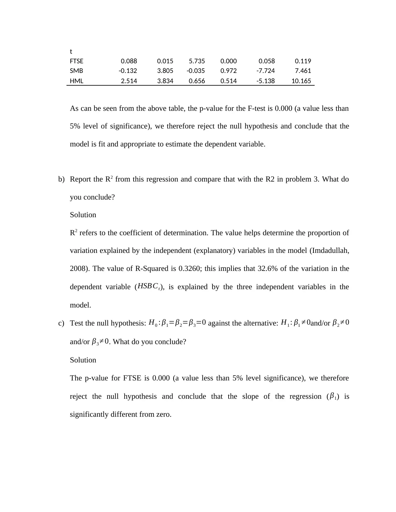
a) Run the regression: [ HSB Ct −r f , t ]= β0 + β1 [ FTSE 100t −r f ,t ]+β2 HM Lt + β 3 SM Bt +εt and
interpret the regression results.
Solution
SUMMARY OUTPUT
Regression Statistics
Multiple R 0.570993
R Square 0.326032
Adjusted R Square 0.296299
Standard Error 69.81214
Observations 72
ANOVA
df SS MS F
Significance
F
Regression 3 160321.9 53440.62 10.96502 5.83E-06
Residual 68 331414 4873.735
Total 71 491735.8
Coefficient
s
Standard
Error t Stat P-value
Lower
95%
Upper
95%
Intercep 34.905 101.359 0.344 0.732 -167.355 237.164

t
FTSE 0.088 0.015 5.735 0.000 0.058 0.119
SMB -0.132 3.805 -0.035 0.972 -7.724 7.461
HML 2.514 3.834 0.656 0.514 -5.138 10.165
As can be seen from the above table, the p-value for the F-test is 0.000 (a value less than
5% level of significance), we therefore reject the null hypothesis and conclude that the
model is fit and appropriate to estimate the dependent variable.
b) Report the R2 from this regression and compare that with the R2 in problem 3. What do
you conclude?
Solution
R2 refers to the coefficient of determination. The value helps determine the proportion of
variation explained by the independent (explanatory) variables in the model (Imdadullah,
2008). The value of R-Squared is 0.3260; this implies that 32.6% of the variation in the
dependent variable (HSB Ct), is explained by the three independent variables in the
model.
c) Test the null hypothesis: H0 : β1=β2=β3=0 against the alternative: H1 : β1 ≠ 0and/or β2 ≠ 0
and/or β3 ≠ 0. What do you conclude?
Solution
The p-value for FTSE is 0.000 (a value less than 5% level significance), we therefore
reject the null hypothesis and conclude that the slope of the regression ( β1) is
significantly different from zero.

The p-value for SMB is 0.972 (a value greater than 5% level significance), we therefore
fail to reject the null hypothesis and conclude that the slope of the regression ( β2) is not
significantly different from zero.
The p-value for HML is 0.514 (a value greater than 5% level significance), we therefore
fail to reject the null hypothesis and conclude that the slope of the regression ( β3) is not
significantly different from zero.
d) Test the null hypothesis: H0 : β1=1 and β3=0 against the alternative H1 : β1 ≠1 and/or
β3 ≠ 0. What do you conclude?
Solution
The p-value for FTSE is 0.000 (a value less than 5% level significance), we therefore
reject the null hypothesis and conclude that the slope of the regression ( β1) is
significantly different from zero.
The p-value for SMB is 0.972 (a value greater than 5% level significance), we therefore
fail to reject the null hypothesis and conclude that the slope of the regression ( β2) is not
significantly different from zero (Armstrong, 2012).
The p-value for HML is 0.514 (a value greater than 5% level significance), we therefore
fail to reject the null hypothesis and conclude that the slope of the regression ( β3) is not
significantly different from zero (Tofallis, 2009).
e) Obtain a plot of the residuals for this regression. What can you tell about the residuals?
Solution

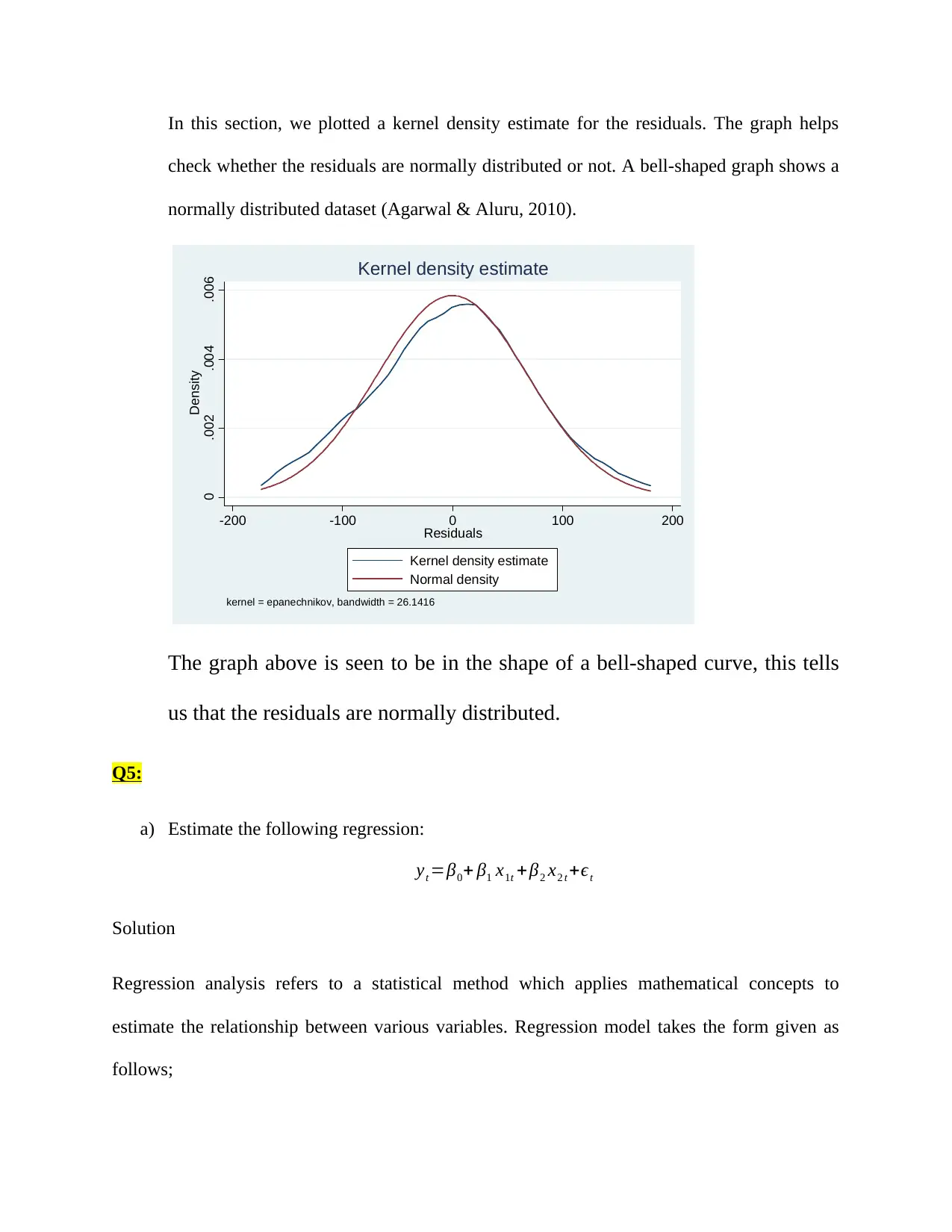
In this section, we plotted a kernel density estimate for the residuals. The graph helps
check whether the residuals are normally distributed or not. A bell-shaped graph shows a
normally distributed dataset (Agarwal & Aluru, 2010).
0 .002 .004 .006
Density
-200 -100 0 100 200
Residuals
Kernel density estimate
Normal density
kernel = epanechnikov, bandwidth = 26.1416
Kernel density estimate
The graph above is seen to be in the shape of a bell-shaped curve, this tells
us that the residuals are normally distributed.
Q5:
a) Estimate the following regression:
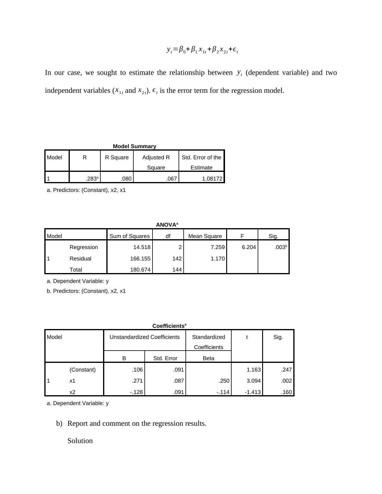
yt =β0+ β1 x1t +β2 x2 t +ϵt
Solution
Regression analysis refers to a statistical method which applies mathematical concepts to
estimate the relationship between various variables. Regression model takes the form given as
follows;

yt =β0+ β1 x1t +β2 x2 t +ϵt
In our case, we sought to estimate the relationship between yt (dependent variable) and two
independent variables ( x1 t and x2 t). ϵt is the error term for the regression model.
Model Summary
Model R R Square Adjusted R
Square
Std. Error of the
Estimate
1 .283a .080 .067 1.08172
a. Predictors: (Constant), x2, x1
ANOVAa
Model Sum of Squares df Mean Square F Sig.
1
Regression 14.518 2 7.259 6.204 .003b
Residual 166.155 142 1.170
Total 180.674 144
a. Dependent Variable: y
b. Predictors: (Constant), x2, x1
Coefficientsa
Model Unstandardized Coefficients Standardized
Coefficients
t Sig.
B Std. Error Beta
1
(Constant) .106 .091 1.163 .247
x1 .271 .087 .250 3.094 .002
x2 -.128 .091 -.114 -1.413 .160
a. Dependent Variable: y
b) Report and comment on the regression results.
Solution

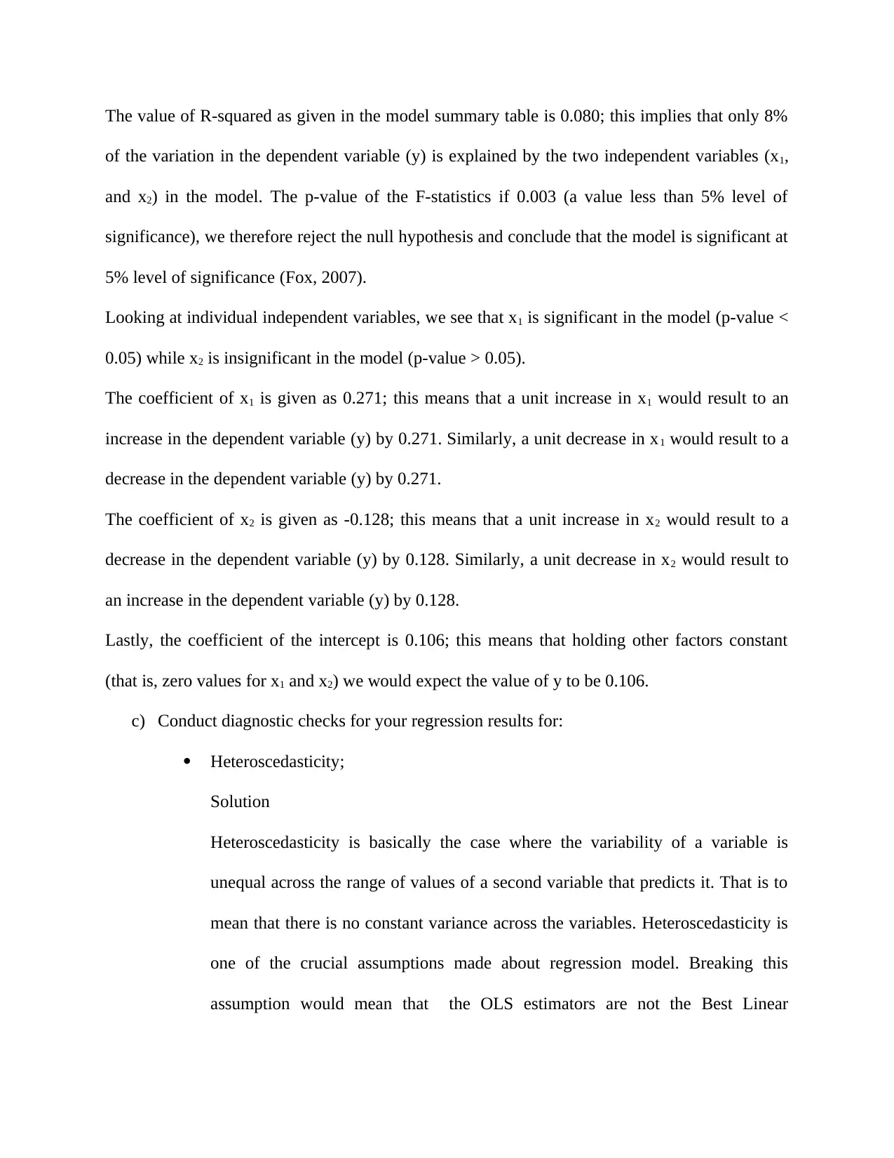
The value of R-squared as given in the model summary table is 0.080; this implies that only 8%
of the variation in the dependent variable (y) is explained by the two independent variables (x1,
and x2) in the model. The p-value of the F-statistics if 0.003 (a value less than 5% level of
significance), we therefore reject the null hypothesis and conclude that the model is significant at
5% level of significance (Fox, 2007).
Looking at individual independent variables, we see that x1 is significant in the model (p-value <
0.05) while x2 is insignificant in the model (p-value > 0.05).
The coefficient of x1 is given as 0.271; this means that a unit increase in x1 would result to an
increase in the dependent variable (y) by 0.271. Similarly, a unit decrease in x1 would result to a
decrease in the dependent variable (y) by 0.271.
The coefficient of x2 is given as -0.128; this means that a unit increase in x2 would result to a
decrease in the dependent variable (y) by 0.128. Similarly, a unit decrease in x2 would result to
an increase in the dependent variable (y) by 0.128.
Lastly, the coefficient of the intercept is 0.106; this means that holding other factors constant
(that is, zero values for x1 and x2) we would expect the value of y to be 0.106.
c) Conduct diagnostic checks for your regression results for:
 Heteroscedasticity;
Solution
Heteroscedasticity is basically the case where the variability of a variable is
unequal across the range of values of a second variable that predicts it. That is to
mean that there is no constant variance across the variables. Heteroscedasticity is
one of the crucial assumptions made about regression model. Breaking this
assumption would mean that the OLS estimators are not the Best Linear

Unbiased Estimators (BLUE) and their variance is not the lowest of all other
unbiased estimators.
Prob > chi2 = 0.0000
chi2(1) = 80.08
Variables: fitted values of y
Ho: Constant variance
Breusch-Pagan / Cook-Weisberg test for heteroskedasticity
. hettest
Applying hettest command in stata, we sought to check for heteroscedasticity
using Breusch-Pagan test. Results showed that the p-value of the test was 0.000 (a
value less than 5% level of significance), we therefore reject the null hypothesis
of constant variance and conclude that the regression results are not
homoscedastic (no equal variance).
 Autocorrelation (1st order and 12th order);
Solution
Autocorrelation also known as serial correlation is the correlation that exists
between a time series with its own past and future values. It could also refer to the
correlation between members of a series of numbers arranged in time.
Durbin-Watson d-statistic( 3, 0) = .
. estat dwatson
Results on autocorrelation are inconclusive since the p-value was not obtained
from the results hence it is not possible to determine whether there is serial
autocorrelation or not.
 Normality
Solution

This is another crucial assumption that needs to be made regarding data before
running a regression model. Normality refers to the modeling of data in a normal
distribution.
r 144 0.90692 10.459 5.310 0.00000
Variable Obs W V z Prob>z
Shapiro-Wilk W test for normal data
. swilk r
Using Shapiro-Wilk test, we checked whether the regression results were
normally distributed. The p-value of the test was found to be 0.000 (a value less
than 5% level of significance), we therefore reject the null hypothesis of
normality and conclude that the regression results are not normally distributed at
5% level of significance.
d) Are there any issues? How do you suggest fixing them?
Solution
Yes are there issues to do with the regression results. Some of the issues are;
 Non-normality of the data
 Heteroscedasticity of the dataset
With the above problems, the results are bound to be biased and not reflect the true
results. Hence the issues need to be fixed. For the heteroscedasticity, a robust regression
need to be performed instead of the standard regression. For the non-normality, a set of
transformations need to be performed to ensure normality of the dataset.

References
Armstrong, J. S., 2012. Illusions in Regression Analysis. International Journal of Forecasting
(forthcoming), 28(3), p. 689.
Fox, J., 2007. Applied Regression Analysis, Linear Models and Related Methods.
Gigerenzer, G., 2004. Mindless statistics. Journal of Socio-Economics, 33(5), p. 587–606.
Hinkelmann, K. & Kempthorne, O., 2008. Design and Analysis of Experiments. I and II.
Rubin, D. B. & Little, R. J. A., 2012. Statistical analysis with missing data.
Tabachnick, B. G. & Fidell, L. S., 2007. Using Multivariate Statistics.
Tofallis, C., 2009. Least Squares Percentage Regression. Journal of Modern Applied Statistical
Methods, 7(5), p. 526–534.

Appendix: