Examining Day's Hypothesis on Müller-Lyer Illusion

This study examines Day's hypothesis on the Müller-Lyer illusion and conflicting cues created by global and local features. Participants were split into three groups: Global processing condition, Local processing condition, and Control group. Results show the illusion is more severe in the global group and weaker in the local group. No significant difference in slope adjustments was found across the three groups. A total of 322 participants took part in the experiment. The study also explores the relationship between gender, age, and slope adjustments.

Running Head: DATA ANALYSIS 1
Data Analysis
Name:
Institution:
14th April 2018

DATA ANALYSIS 2
Abstract
This study sought to carry out a novel and innovative study to examine Day’s hypothesis that the
Müller-Lyer illusion is created by ‘conflicting cues’ created by global and local features.
Participants were split into three groups or ‘levels of processing’: Global processing condition,
Local processing condition and the control group. A total of 322 participants took part in this
experiment with majority (75%) being female participants. The average age of the participants
was 21.82 years old. Results showed that Global had a steeper regression line compared with
Control which implied that the visual illusion had become more severe therefore producing
greater adjustment errors while on the other hand the local had a more shallow regression line
compared with Control indicating that the illusion had weakened thus creating fewer errors.
However, the slope adjustments were found not to be significantly different across the three
groups (Global, Local and Control groups).
Introduction

DATA ANALYSIS 3
In the Müller-Lyer illusion the right vertical line (see the figure above) appears to be longer than
the left vertical line, even though they are both exactly the same length. The presence of the fins
at either end makes the lines appear to be different in length, with the fins-in arrangement
causing the left line to look shorter and the fins-out arrangement causing the right line to look
longer. Müller-Lyer coined the term "confluxion" to describe this illusion ("Müller-Lyer," n.d.).
The exact nature of this effect has been studied extensively without consensus (c.f., Dewar,
1967; Presey & Martin, 1990; Restle & Decker, 1977) about which perceptual principles account
for the illusion ("Müller-Lyer," n.d.).
In order to replicate and extend the findings of Mundy (2014), we have selected an alternative
method of generating global and local bias - mood induction. It has been shown by a number of
researchers (e.g., Gasper & Clore, 2002) that mood has a significant bearing on perception. Sad
people tend to favour processing of local features, whereas happy people tend to prefer
processing whole (global) stimuli. Moreover, it has also been shown that listening to music can
alter your mood. So, if we listen to some happy music, do we become more susceptible to the
Muller-Lyer illusion, since our perceptual system is now biased more globally? On the other
hand, if we listen to sad music, do we see the illusion more weakly, due to enhanced local
processing? You should do a literature search to find more examples of this mood-perception
phenomenon - there are a number within the face processing literature (e.g., Hills & Lewis,
2011) and further afield.

DATA ANALYSIS 4
Methodology
Stage 1
The class will split into three groups or ‘levels of processing’:
1. Global processing condition (Happy Mood Induction) - https://youtu.be/LYHPKkIHytA
2. Local processing condition (Sad Mood Induction) - https://youtu.be/sPlhKP0nZII
Control condition
Participants in groups 1 and 2 will listen to pre-determined music 1 minute before and during the
entire experiment. The Global participants will listen to Mozart Jubilate and Exultate to induce a
happy mood; the Local participants will listen to Mozart Requiem to induce a sad mood (music
was chosen from examples given in Hills, Werno and Lewis (2011)). The Control participants
will not listen to music before and during the experiment.
Stage 2
All participants will now access the experiment URL and enter their class ID code according to
which condition they are in. The study contained in this URL is a variation of the original
Muller-Lyer illusion, one which enables investigators to study the effect of changes in fin angle
on the apparent length of lines. Participants in the study are presented with two lines, as in the
standard Muller-Lyer illusion presentation, but one of the lines has fins and one does not.
Moreover, the two lines are initially different in length. The participant's task is to adjust the
plain line (without fins) to make the lengths the same. The adjustment is made using a slider

DATA ANALYSIS 5
(arrow in the figure below) that can be dragged using the computer mouse. As the slider is
moved up and down the scale, the adjustable line changes in length.
Participant’s demographic
A total of 322 respondents took part in the study with majority being female participants. The
mean age for the participants was 21.82 with a median age being 21 years old. The participants
voluntarily participated in the study without being coerced in any way.
Table 1: Participant Demographic Statistics
Age Range 18-52
Median Age 21
Mean Age for all Participants 21.82
Standard Deviation for all
Participants
4.33
Total Number of Participants (N) 322
Split By Sex
Mean Age for all Women 21.81
Standard Deviation for all Women 4.37
Total Number of Women (N) 242
Mean Age for all Men 21.85
Standard Deviation for all Men 4.37
Total Number of Men (N) 80
Results and findings
Examination of data
A scatter plot of Adjustment errors against Fin angle was plotted in order to investigate the effect
of fin angle on adjustment error. The figure below is a plot of data points that represent how the

DATA ANALYSIS 6
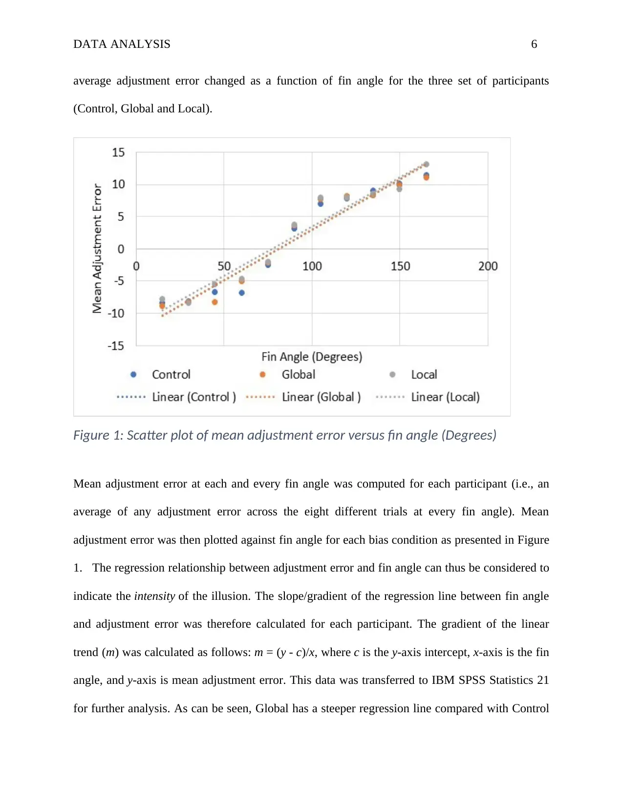
average adjustment error changed as a function of fin angle for the three set of participants
(Control, Global and Local).
Figure 1: Scatter plot of mean adjustment error versus fin angle (Degrees)
Mean adjustment error at each and every fin angle was computed for each participant (i.e., an
average of any adjustment error across the eight different trials at every fin angle). Mean
adjustment error was then plotted against fin angle for each bias condition as presented in Figure
1. The regression relationship between adjustment error and fin angle can thus be considered to
indicate the intensity of the illusion. The slope/gradient of the regression line between fin angle
and adjustment error was therefore calculated for each participant. The gradient of the linear
trend (m) was calculated as follows: m = (y - c)/x, where c is the y-axis intercept, x-axis is the fin
angle, and y-axis is mean adjustment error. This data was transferred to IBM SPSS Statistics 21
for further analysis. As can be seen, Global has a steeper regression line compared with Control

DATA ANALYSIS 7
which shows that the visual illusion has become more severe therefore producing greater
adjustment errors while on the other hand the local has a more shallow regression line compared
with Control indicating that the illusion has weakened thus creating fewer errors.
Descriptive Statistics
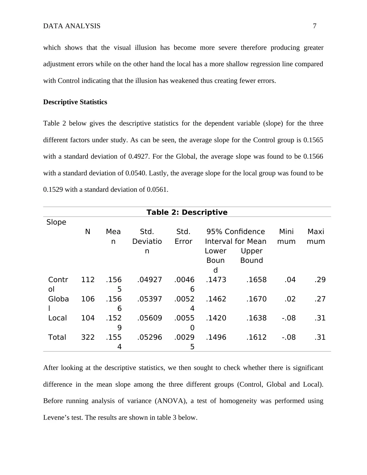
Table 2 below gives the descriptive statistics for the dependent variable (slope) for the three
different factors under study. As can be seen, the average slope for the Control group is 0.1565
with a standard deviation of 0.4927. For the Global, the average slope was found to be 0.1566
with a standard deviation of 0.0540. Lastly, the average slope for the local group was found to be
0.1529 with a standard deviation of 0.0561.
Table 2: Descriptive
Slope
N Mea
n
Std.
Deviatio
n
Std.
Error
95% Confidence
Interval for Mean
Mini
mum
Maxi
mum
Lower
Boun
d
Upper
Bound
Contr
ol
112 .156
5
.04927 .0046
6
.1473 .1658 .04 .29
Globa
l
106 .156
6
.05397 .0052
4
.1462 .1670 .02 .27
Local 104 .152
9
.05609 .0055
0
.1420 .1638 -.08 .31
Total 322 .155
4
.05296 .0029
5
.1496 .1612 -.08 .31
After looking at the descriptive statistics, we then sought to check whether there is significant
difference in the mean slope among the three different groups (Control, Global and Local).
Before running analysis of variance (ANOVA), a test of homogeneity was performed using
Levene’s test. The results are shown in table 3 below.

DATA ANALYSIS 8
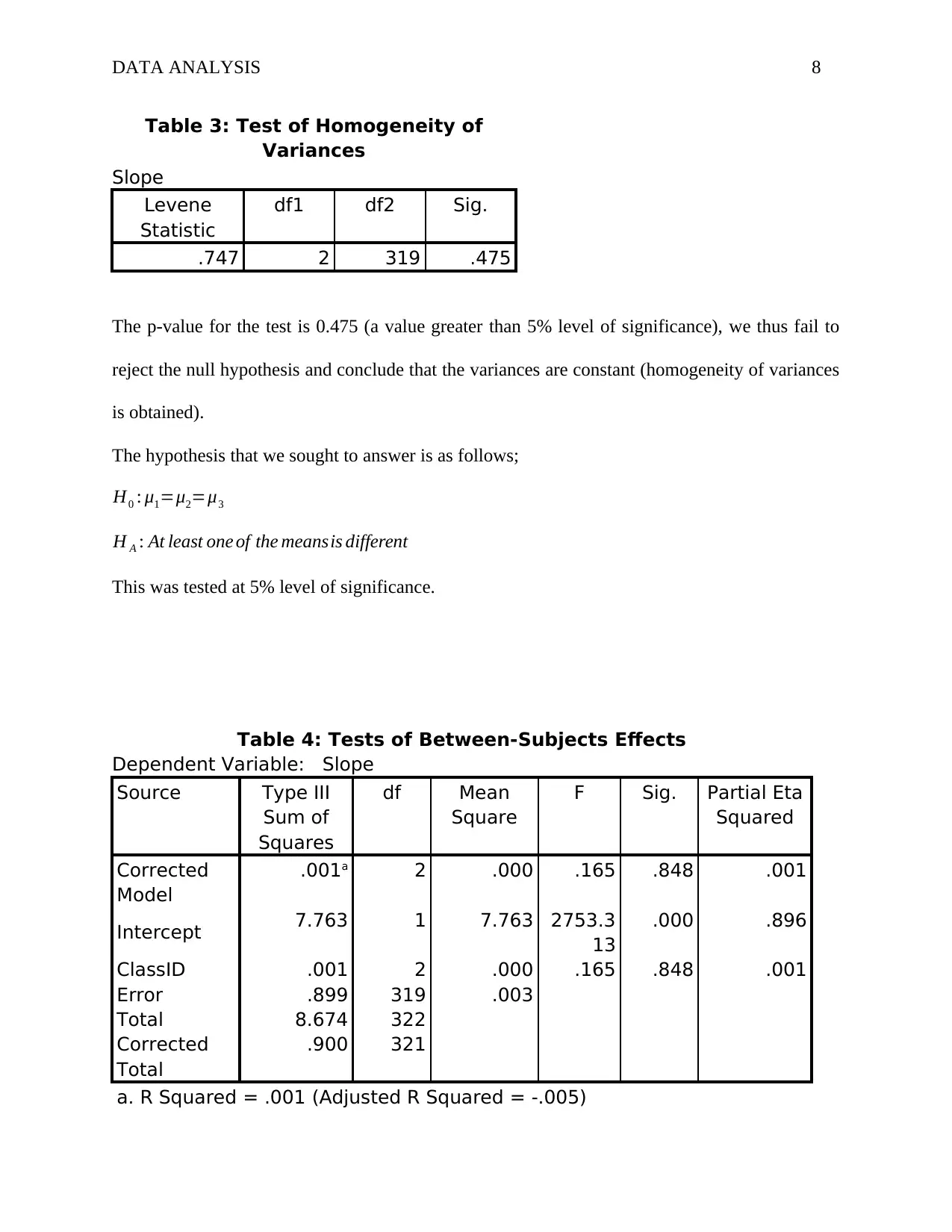
Table 3: Test of Homogeneity of
Variances
Slope
Levene
Statistic
df1 df2 Sig.
.747 2 319 .475
The p-value for the test is 0.475 (a value greater than 5% level of significance), we thus fail to
reject the null hypothesis and conclude that the variances are constant (homogeneity of variances
is obtained).
The hypothesis that we sought to answer is as follows;
H0 : μ1=μ2=μ3
H A : At least one of the meansis different
This was tested at 5% level of significance.
Table 4: Tests of Between-Subjects Effects
Dependent Variable: Slope
Source Type III
Sum of
Squares
df Mean
Square
F Sig. Partial Eta
Squared
Corrected
Model
.001a 2 .000 .165 .848 .001
Intercept 7.763 1 7.763 2753.3
13
.000 .896
ClassID .001 2 .000 .165 .848 .001
Error .899 319 .003
Total 8.674 322
Corrected
Total
.900 321
a. R Squared = .001 (Adjusted R Squared = -.005)

DATA ANALYSIS 9
As can be seen, the p-value is 0.848 (a value greater than 5% level of significance), we thus fail
to reject the null hypothesis and conclude that there is no significant difference in the mean slope
for the different groups (Local, Control and Global groups).
Is there significant difference in the slope between males and females?
In this section, the study sought to understand how gender (males and females) compare in terms
of the slope. The hypothesis tested is as follows;
H0: There is no significant difference in the mean slope for the males and females
HA: There is significant difference in the mean slope for the males and females
This was tested at 5% level of significance.
The results of the independent samples t-test is shown in the tables below;
Table 5:Group Statistics
sex N Mean Std.
Deviation
Std. Error
Mean
Slop
e
Male 80 .1424 .05321 .00595
Femal
e
242 .1597 .05228 .00336
Table 5 shows that the average slope is 0.1424 for the male respondents and 0.11597 for the
female respondents with standard deviations of 0.0532 and 0.0523 respectively.
Table 6:Independent Samples Test
Levene's Test for
Equality of
Variances
t-test for Equality of Means

DATA ANALYSIS 10
F Sig. t df Sig. (2-
tailed)
Mean
Differen
ce
Std.
Error
Differen
ce
95% Confidence
Interval of the
Difference
Lower Upper
Slope
Equal variances
assumed
.017 .895 -2.543 320 .011 -.01722 .00677 -.03055 -.00390
Equal variances
not assumed
-2.520 133.022 .013 -.01722 .00683 -.03074 -.00371
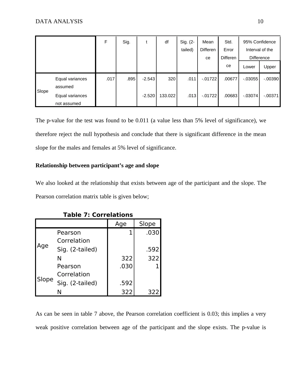
The p-value for the test was found to be 0.011 (a value less than 5% level of significance), we
therefore reject the null hypothesis and conclude that there is significant difference in the mean
slope for the males and females at 5% level of significance.
Relationship between participant’s age and slope
We also looked at the relationship that exists between age of the participant and the slope. The
Pearson correlation matrix table is given below;
Table 7: Correlations
Age Slope
Age
Pearson
Correlation
1 .030
Sig. (2-tailed) .592
N 322 322
Slope
Pearson
Correlation
.030 1
Sig. (2-tailed) .592
N 322 322
As can be seen in table 7 above, the Pearson correlation coefficient is 0.03; this implies a very
weak positive correlation between age of the participant and the slope exists. The p-value is

DATA ANALYSIS 11
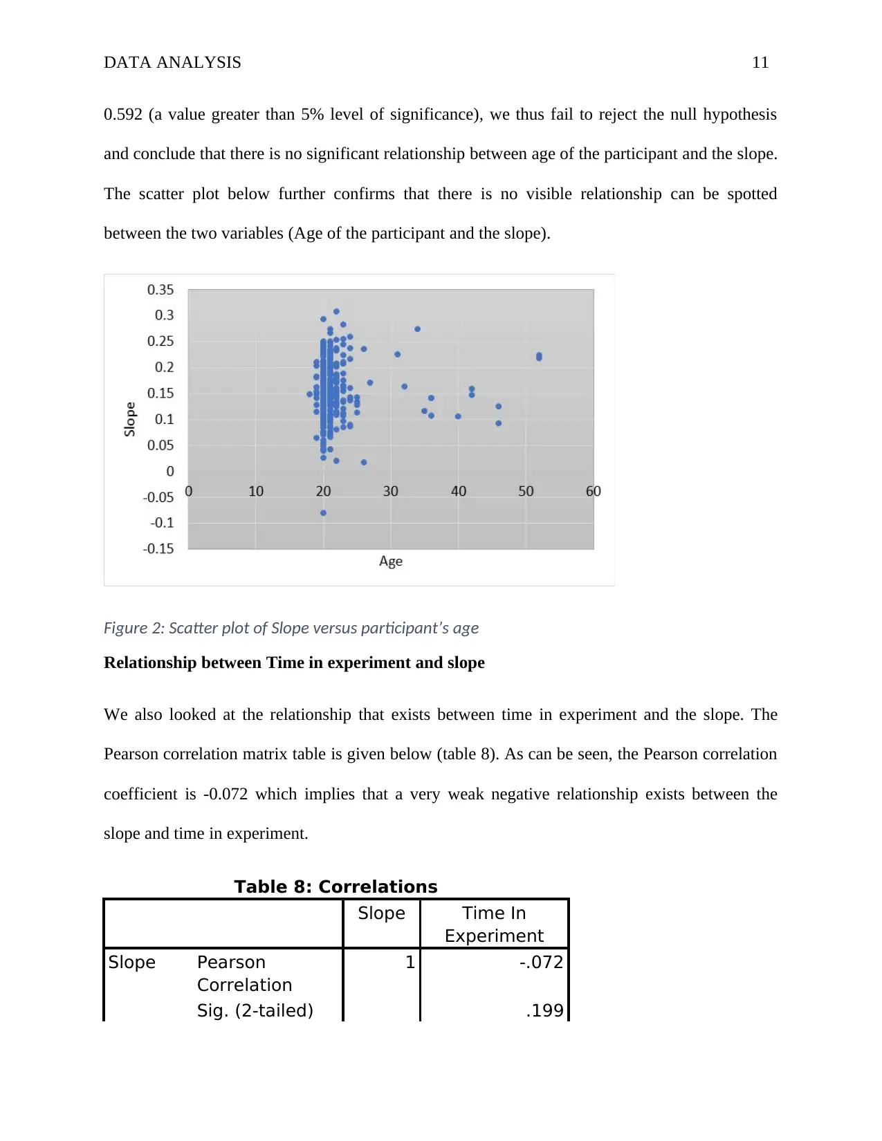
0.592 (a value greater than 5% level of significance), we thus fail to reject the null hypothesis
and conclude that there is no significant relationship between age of the participant and the slope.
The scatter plot below further confirms that there is no visible relationship can be spotted
between the two variables (Age of the participant and the slope).
Figure 2: Scatter plot of Slope versus participant’s age
Relationship between Time in experiment and slope
We also looked at the relationship that exists between time in experiment and the slope. The
Pearson correlation matrix table is given below (table 8). As can be seen, the Pearson correlation
coefficient is -0.072 which implies that a very weak negative relationship exists between the
slope and time in experiment.
Table 8: Correlations
Slope Time In
Experiment
Slope Pearson
Correlation
1 -.072
Sig. (2-tailed) .199

DATA ANALYSIS 12
N 322 322
Time In
Experime
nt
Pearson
Correlation
-.072 1
Sig. (2-tailed) .199
N 322 322
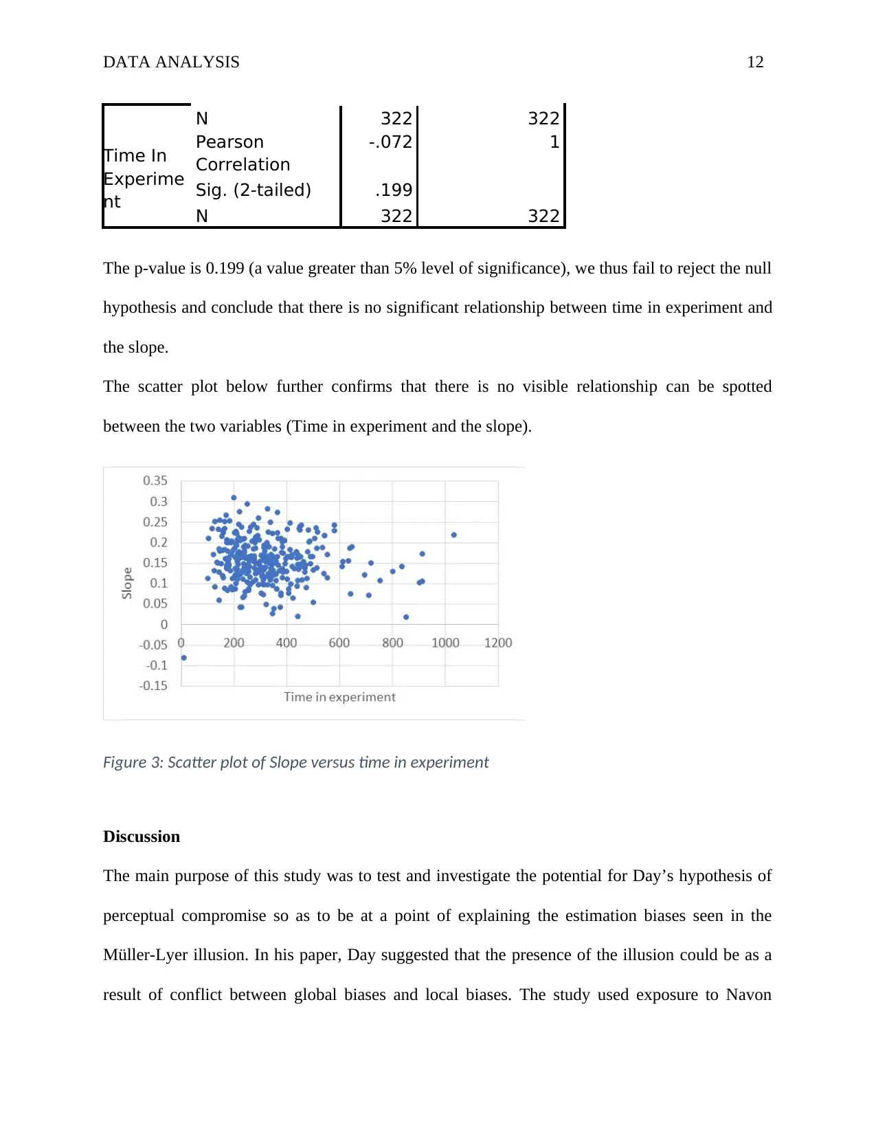
The p-value is 0.199 (a value greater than 5% level of significance), we thus fail to reject the null
hypothesis and conclude that there is no significant relationship between time in experiment and
the slope.
The scatter plot below further confirms that there is no visible relationship can be spotted
between the two variables (Time in experiment and the slope).
Figure 3: Scatter plot of Slope versus time in experiment
Discussion
The main purpose of this study was to test and investigate the potential for Day’s hypothesis of
perceptual compromise so as to be at a point of explaining the estimation biases seen in the
Müller-Lyer illusion. In his paper, Day suggested that the presence of the illusion could be as a
result of conflict between global biases and local biases. The study used exposure to Navon

DATA ANALYSIS 13
stimuli to create a bias in processing level, that is, either local bias or global bias before testing
the illusory strength of the Müller-Lyer illusion. Unlike the results by Mundy (2014), the study
did not get significant effect of the biases though global bias had a slightly higher slope.
Analysis of the three groups in terms of their slope comparison was conducted. The main effect
of facial expression and the interaction were not significant: F(2, 319) = 0.17, MSE = 0.07, p
= .85, ηp
2 =0.001 .Happy mood induction participants (M = 0.16, SD = 0.05) had a more average
slope than sad mood induction participants (M = 0.15, SD = 0.06) and participants with control
bias (M = 0.16, SD = 0.05), although no differences were significant.
An independent samples t-test was performed to compare the mean slope for the male and the
female students in the study. Results showed that the average slope for the female participants
(M = 0.16, SD = 0.05, N = 242) was significantly different (higher) than the average slope for
the male participants (M = 0.14, SD = 0.05, N = 80), t (320) = -2.54, p < .05, two-tailed. The
difference of -0.02 showed a significant difference. Essentially results showed that the female
participants had significantly higher slopes as compared to the male participants in the same
environment.
A Pearson product-moment correlation coefficient was computed to assess the relationship
between the age of the participants and the slope. There was an insignificant weak positive
correlation between the two variables, r = 0.03, n = 322, p = 0.592. Lastly, A Pearson product-
moment correlation coefficient was computed to assess the relationship between the time in
experiment and the slope. There was an insignificant weak negative correlation between the two
variables, r = -0.07, n = 322, p = 0.199.

DATA ANALYSIS 14
References
Hills, P. J. & Lewis, M. B. (2011). Sad people avoid the eyes or happy people focus on the eyes?
Mood induction affects facial feature discrimination. British Journal of Psychology, 102(2), 260-
274.
Hills, P.J., Werno, M.A., & Lewis, M.B. (2011). Sad people are more accurate at face
recognition than happy people. Consciousness and Cognition, 20, 1502-1517.
Macrae, C.N. & Lewis, H.L. (2002). Do I know you? Processing orientation and face
recognition. Psychological Science, 13, 194-196.
Müller-Lyer. (n.d.). Online Psychological Laboratory. Retrieved
from http://opl.apa.org/Experiments/About/AboutM%C3%BCller-Lyer.aspx.
Mundy, M.E. (2014). Testing day: The effects of processing bias induced by Navon stimuli on
the strength of the Muller-Lyer illusion. Advances in Cognitive Psychology, 10, 9-14.
Navon, D. (1977). Forest before the trees: The precedence of global features in visual
perception. Cognitive Psychology, 9, 353-383.
Pressey, A. & Martin, N.S. (1990). The effects of varying fins in Muller-Lyer and holding
illusions. Psychological Research, 52, 46-53.
Restle, F. & Decker, J. (1977). Size of the Muller-Lyer illusions a function of its dimensions:
Theory and data. Perception and Psychophysics, 21, 489-503.